Tutorial¶

This chapter describes step by step how to run the CSO pre-processor and observation operator.

Run script¶

The script to run one-or-more CSO tasks is:

./bin/cso --help

The tasks are configured in text files; the name of the settings file should be passed as first argument:

./bin/cso  config/tutorial/tutorial.rc

The settings file is formatted after an X-resource file, and therefore has extension .rc. For a description of the format, see the section on rcfile formatting in the rc module.

The settings in config/tutorial/tutorial.rc are used in the examples below.

Job tree¶

The configuration defines a series of jobs to be created and started. For example, the following jobs might be defined to process Sentinel-5p data:

cso.tutorial.inquire-scihub
cso.tutorial.convert
cso.tutorial.listing
cso.tutorial.catalogue

This list is actually defined as tree, using lists in which the elements could be a list too:

cso                            # tree with element "tutorial"
   .tutorial                   # tree with elements "inquire-scihub", "convert", "listing", and "catalogue"
            .inquire-scihub    # step
            .convert           # step
            .listing           # step
            .catalogue         # step

For each element in the tree, the configuration file should specify the name of a python class that takes care of the job creating.. If the element is a tree, use the utopya.UtopyaJobTree class, and add a line to specify the names of the sub-elements. For the main cso job, this looks like:

! class to create a job tree:
cso.class                           :  utopya.UtopyaJobTree
! list of sub-elements:
cso.elements                        :  tutorial

In this example, the main job has only one sub-job. The name of a sub-job is a concatenation of the element names using dots:

cso.tutorial

Also for this name a class name should be defined that takes care of the job creation; in this example again a tree is defined:

! class to create a job tree:
cso.tutorial.class                       :  utopya.UtopyaJobTree
! list of sub-elements:
cso.tutorial.elements                    :  inquire-scihub convert listing catalogue

A job that is no container for sub-jobs but should actually do some work should be defined with the utopya.UtopyaJobStep class. This is for example the case for the cso.tutorial.inquire-scihub job:

! single step:
cso.tutorial.inquire-scihub.class          :  utopya.UtopyaJobStep

A job step will perform at least one task to do the actual work. A task should be specified by the name of a python class that should do the work, and the the arguments that should be passed to initialize it. The following task description is a dummy that can be used for testing, it will only print a message:

! dummy task:
cso.tutorial.inquire-scihub.task.class     :  utopya.UtopyaJobTask
cso.tutorial.inquire-scihub.task.args      :  msg='Inquire SciHub ...'

Running a single job step¶

To just run a single job step from the tree, specify the name and a special flag:

./bin/cso  config/tutorial/tutorial.rc  --rcbase='cso.tutorial.listing'  --single

Job files¶

The job tree defined above will create a series of job files in a work directory, with each job in a separate sub directory:

/work/yourname/CSO-Tests/cso/cso.jb
                         cso/tutorial/cso.s5p.jb
                         cso/tutorial/inquire-scihub/cso.tutorial.inquire-scihub.jb

The location of the work directories is specified in the settings using:

! work directory for jobs;
! here path including subdirectories for job name elements:
*.workdir                           :  /work/yourname/CSO-Tests/__NAME2PATH__

The default settings create simple job files that will run in foreground, perform a specified task, and submit the next job in the tree. However, with more detailed settings it also possible to create job files that:

contain batch job settings, and are submitted to a queue system (slurm, pbs, lsf, …);
load environment modules to setup library paths etc;
include user defined lines for fine tuning.

See the documentation of the utopya_jobtree module for the advanced settings.

Step 1 - Inquire S5p archive¶

(See Inquire Sentinel-5p/NO2 archives section for full description of S5p/NO2 inquireries)

The cso.tutorial.inquire-scihub job is configured in rc/tutorial.rc to crawl the Copernicus SciHub archive for available Sentinel-5p NO2 observations.

Important

Access to the Copernicus Open Access Hub requires a (not personal) login and password; see also the Open Hub section. Add the following login/password setting to your ~/.netrc file:

machine s5phub.copernicus.eu    login s5pguest     password s5pguest

To run the inquire job only, limit the element list of the cso.tutorial job to:

cso.tutorial.elements               :  inquire-scihub

The job configuration defines that should perform two tasks: first create a table file with information on the available orbits, and second to create a plot to illustrate the available observations:

! single step:
cso.tutorial.inquire-scihub.class              :  utopya.UtopyaJobStep
! two tasks:
cso.tutorial.inquire-scihub.tasks              :  table plot
!~ inquire available files:
cso.tutorial.inquire-scihub.table.class        :  cso.CSO_SciHub_Inquire
cso.tutorial.inquire-scihub.table.args         :  '${PWD}/config/tutorial/tutorial.rc', \
                                                      rcbase='cso.tutorial.inquire-s5phub-table'
!~ create plot of available versions:
cso.tutorial.inquire-scihub.plot.class         :  cso.CSO_SciHub_InquirePlot
cso.tutorial.inquire-scihub.plot.args          :  '${PWD}/config/tutorial/tutorial.rc', \
                                                      rcbase='cso.tutorial.inquire-s5phub-plot'

The first setting defines that this is single job step that should do some work.

The tasks list defines keywords for the two tasks to be performed.

For the table task, define that the CSO_SciHub_Inquire class should be used to do the work; the class is accessible from the cso module (implemented in``py/cso.py``). The arguments that initialize the class specify the name of an rcfile with settings (tutorial-s5p.rc) and that the settings start with keywords 'cso.tutorial.inquire-s5phub-table'.
Similar for the plot task, the settings define that the CSO_SciHub_InquirePlot class should be used to do the work.

The tutorial settings will inquire the time range 2018-2021.

An important configuration setting that might need to changed is the base location for the work directories. This is specified with a user defined keyword, here chosen to start with ‘my.’:

! base location for work directories:
my.work                         :  /work/${USER}/CSO-Tests

This user defined key is for example used to specify the work directory of the cso.tutorial.inquire-scihub (and other) jobs:

! work directory for jobs;
! here path including subdirectories for job name elements:
*.workdir                           :  ${my.work}/__NAME2PATH__

This tells that the work directory of the job should include the jobname expanded as subdirectories. For this example, the full path becomes:

/work/yourname/CSO-Tests/cso/tutorial/inquire-scihub/

The base of the work directories is also used to specify where the inquired table file should be stored:

! output table, date of today:
cso.tutorial.inquire-s5phub-table.output.file    :  ${my.work}/Copernicus/Copernicus_S5p_NO2_s5phub_%Y-%m-%d.csv

The created table is then for example:

/work/yourname/CSO-Tests/Copernicus/Copernicus_S5p_NO2_s5phub_2022-08-26.csv

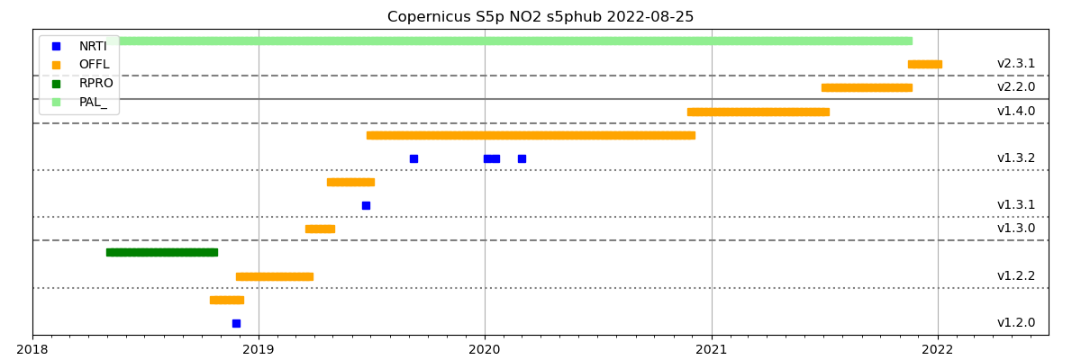
To visualize what is available from the various portals, the cso_scihub.CSO_SciHub_InquirePlot could be used to create an overview figure. The figure file has the base name of the table:

/work/yourname/CSO-Tests/Copernicus/Copernicus_S5p_NO2_s5phub_2022-08-26.png

and looks like:

Overview of available NO2 processings on SciHub.

Step 2 - Convert to CSO format¶

(See Conversion to CSO format section for full description of S5p/NO2 conversion)

The cso.tutorial.convert job is configured to convert the downloaded orbit files into a common format. The conversion includes filter options to selected only pixels within a certain domain, and with some minimum quality flag, etc; this could strongly limit the data volume.

To run the conversion job only, limit in rc/tutorial.rc the element list of the cso.tutorial job to:

cso.tutorial.elements               :  convert

The conversion job is configured with:

! single step:
cso.tutorial.convert.class           :  utopya.UtopyaJobStep
! conversion task:
cso.tutorial.convert.task.class      :  cso.CSO_S5p_Convert
cso.tutorial.convert.task.args       :  '${PWD}/config/tutorial/tutorial-s5p.rc', \
                                         rcbase='cso.tutorial.convert'

The conversion is thus done using the CSO_S5p_Convert class that can be accessed from the cso module. The arguments that initialize the class specify the name of an rcfile with settings (tutorial-s5p.rc) and that the settings start with keywords 'cso.tutorial.convert'.

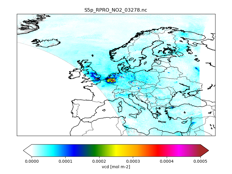
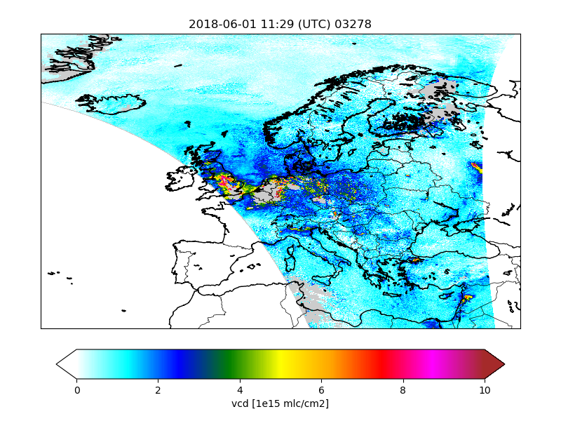
The result of the conversion is a set of files holding the selected pixels per orbit:

/work/yourname/CSO-Tests/CSO-data/S5p/RPRO/NO2/CAMS/2018/06/S5p_RPRO_NO2_03272.nc
                                                            S5p_RPRO_NO2_03273.nc
                                                            :

The configuration of the convert task describes which selection criteria should be applied, which variables should be created in the output files, and how these should be formed.

Step 3 - Example plot¶

The CSO tools could be made in a Python code to read and plot the converted data. The following is a demo Python code that creates an S5p/NO2 map:

#! /usr/bin/env python

"""
Demo for how to read and plot NO2 map from S5p data converted by CSO.
"""

# modules:
import os
import matplotlib.pyplot as plt

# tools:
import cso

# sample file:
filename = '/work/yourname/CSO-Tests/CSO-data/S5p/RPRO/NO2/CAMS/2018/06/S5p_RPRO_NO2_03278.nc'

# read:
orb = cso.CSO_File( filename=filename )

# variable:
vname = 'vcd' ; vmax = 0.0005 # vertical column density
# extract corner grids and values:
xx,yy,values,attrs = orb.GetTrack( vname )

# map domain west/east/south/north:
domain = [-30,45,30,76]
# annote:
title = os.path.basename(filename)
label = '%s [%s]' % (vname,attrs['units'])
# create map figure (single layer):
fig = cso.QuickMap( values[:,:,0], xx=xx, yy=yy, vmin=0.0, vmax=vmax,
                          bmp=dict(resolution='l',countries=True,domain=domain,title=title),
                          cbar=dict(label=label), figsize=(8,6) )
# save:
fig.Export( 'S5p_RPRO_NO2_%s_sample.png' % vname )

# show:
plt.show()

Step 4 - Create listing file¶

(See Listing file section for main description)

The cso.tutorial.listing job creates a listing file for the converted orbits:

CSO-data/S5p/listing-NO2-CAMS.csv

The listing csv file contains a table with records for each of created orbit files, the time range of pixels in the file, and for convenience also the orbit number:

filename                                   ;start_time                   ;end_time                     ;orbit
RPRO/NO2/CAMS/2018/06/S5p_RPRO_NO2_03272.nc;2018-06-01T01:32:46.673000000;2018-06-01T01:36:12.948000000;03272
RPRO/NO2/CAMS/2018/06/S5p_RPRO_NO2_03273.nc;2018-06-01T03:12:53.649000000;2018-06-01T03:17:43.082000000;03273
RPRO/NO2/CAMS/2018/06/S5p_RPRO_NO2_03274.nc;2018-06-01T04:52:43.586000000;2018-06-01T04:59:12.377000000;03274
:

This file will be used by the observation operator to selects orbits with pixels valid for a desired time range. Also the catalogue creator described below uses the listing file to select orbits.

The configuration of describes the name of the listing file to be created, and the directories to be scanned for orbit files.

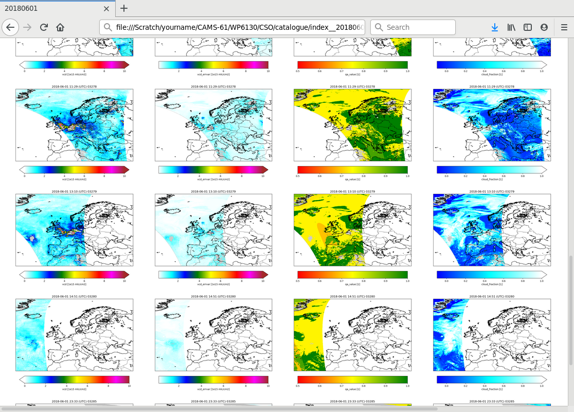
Step 5 - Catalogue of figures¶

(See Catalogue section for main description)

For a first impression of how the downloaded and converted satellite data looks like, the cso.tutorial.catalogue job can be used. This will figures out of the converted files, in particular maps that show values on the track.

To run the catalogue job only, limit in rc/tutorial.rc the element list of the cso.tutorial job to:

cso.tutorial.elements               :  catalogue

The catalogue job consists of two tasks: creation of figures, and creation of index pages to browse through them. This is configured using:

! single step:
cso.tutorial.catalogue.class                   :  utopya.UtopyaJobStep

! two tasks:
cso.tutorial.catalogue.tasks                   :  figs index

! catalogue creation task:
cso.tutorial.catalogue.figs.class              :  cso.CSO_Catalogue
cso.tutorial.catalogue.figs.args               :  '${PWD}/config/tutorial/tutorial-s5p.rc', \
                                                   rcbase='cso.tutorial.catalogue'

! indexer task:
cso.tutorial.catalogue.index.class             :  utopya.Indexer
cso.tutorial.catalogue.index.args              :  '${PWD}/config/tutorial/tutorial-s5p.rc', \
                                                    rcbase='cso.tutorial.catalogue-index'

The figs task that creates the figures uses the CSO_Catalogue class that can be accessed from the cso module. The arguments that initialize the class specify the name of an rcfile with settings (tutorial-s5p.rc) and that the settings start with keywords 'cso.tutorial.catalogue'. The configuration describes where to find a listing file with orbits, which variables should be plot, the colorbar properties, etc.

The names of the created figures is composed from the base name of the converted files and the variable that is plotted:

/work/yourname/CSO-Tests/CSO-data-catalogue/2018/06/01/S5p_RPRO_NO2_03278__vcd.png
                                                       S5p_RPRO_NO2_03278__qa_value.png
                                                       :

Index pages are created to facilitate browsing through the figures. The index is created with the index task of the job. As shown above, the work is done by the Indexer class that can be accessed from the utopya module. The arguments that initialize the class specify the name of an rcfile with settings (tutorial-s5p.rc) and that the settings start with keywords 'cso.tutorial.catalogue-index'.

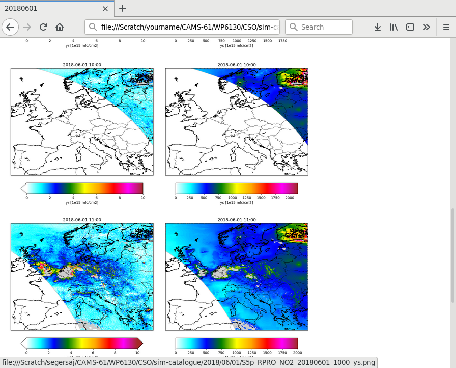
When succesful, the index creator displays an url that could be loaded in a browser:

Browse to:
  file:///work/yourname/CSO-Tests/CSO-data-catalogue/index.html

Step 6 - Demo program for observation operator¶

(See Observation operator section for main description)

The observation operator code consists of Fortran files that should be added to a simulation model. For testing, a dummy program is provided that reads orbit files created by the preprocessor, simulates a (fake) concentration profile, convolves this with the averaging kernels, and writes this to a file as a simulated retrieval.

The code requires that the following is available:

recent Fortran compiler with support for F2008 constructs (for example GFortran v8.2.0)
netCDF library
eventually an MPI wrapper with F2008 interface (for example OpenMPI v4.0.3)

The demo code is included in the subdirectory:

oper/src/Makefile
         :
         tutorial_oper_S5p.F90
     tutorrial_oper_S5p.rc

For testing, copy the entire sub directory to a work directory; configuration assumes a location in the work directory of the pre-processor where the converted orbit files are:

cd /work/yourname/CSO-Tests
cp -r ~/CSO/oper CSO-oper
cd CSO-oper

The steps below describe how to build and run the executable; all steps are included in the following scripts, which might need manual editting for your system!

launcher for serial run;
launcher-mpi for MPI-parallel run.

To compile the code, the following should be used:

cd src/
make tutorial_oper_S5p.x
cd ..

This will probably fail because of incorrect compiler and library settings. Create a copy of the Makefile settings for your own machine:

cd src
cp Makefile_config_template  Makefile_config_institute-machine

Edit the file; for the first tests, do not use mpi-wrappers yet.

Ensure that that Makefile includes the new settings:

include Makefile_config_institute-machine

If with this settings the executable has been compiled successful, run it using:

./src/tutorial_oper_S5p.x

The main program tutorial_oper_S5p.F90 reads settings from the file:

tutorial_oper_S5p.rc

Some of the settings are only needed by the main program, and define a time loop and an assumed simulation domain:

! time range:
tutorial.timerange.start           :  2018-06-01 00:00
tutorial.timerange.end             :  2018-06-02 00:00

! selected domain:
tutorial.domain.west               :  -10
tutorial.domain.east               :   30
tutorial.domain.south              :   35
tutorial.domain.north              :   65

Other settings are needed by the observation operator code. First specify the (relative) location of the listing file with orbit file names and time ranges:

! template for listing with converted files:
tutorial.S5p.no2.listing           : ../CSO-data/S5p/listing-NO2-CAMS.csv

The program will perform a time loop with hourly steps. At every hour, orbits are selected for which the average time falls in the interval of 30 minutes before and after. The observation operator then reads the orbit file, selects the pixels in the model domain, simulates a retrieval, and writes the result to output files.

The operator needs some specific information. For example, tell it to read information on the original tracks too; this will be saved in the output to facilitate creation of map plots:

! also read info on original track (T|F)?
! if enabled, this will be stored in the output too:
tutorial.S5p.no2.with_track        :  T

The current version of the operator will always try to read the following variables from the input files:

retrieved product, denoted as yr;
averaging kernels (A);
pressure interfaces on which the kernel is defined (hp);
retrieval error covariance (vr);
tropospheric airmass facor (M);
tropopause layer index (nla).

This list of variables is specified with:

tutorial.S5p.no2.dvars             :  hp yr vr A M nla

and for each them, detailed settings are specified to know their shape (profile on a priori layers, retrieval layers, matrix) and the name of the variable in the input file:

! half-level pressures:
!~ dimensions, copied from data file:
tutorial.S5p.no2.dvar.hp.dims      :  layeri
!~ source variable:
tutorial.S5p.no2.dvar.hp.source    :  pressure

! retrieval:
!~ dimensions, copied from data file:
tutorial.S5p.no2.dvar.yr.dims      :  retr
!~ source variable:
tutorial.S5p.no2.dvar.yr.source    :  vcd

...

The output that is written for a certain hour when an orbit was available consists of two files:

CSO_output_20180601_0300_data.nc
CSO_output_20180601_0300_state.nc

The data file contains a copy of the original input, limited to the model domain:

footprints of selected pixels (longitudes, latitudes)
footprints of original track;
pressure profiles;
averaging kernels;
retrieved values;
retrieval variance;
optional: horizontal mapping information.

while the state file contains everything related to a simulation:

original model concentration and pressure profiles;
simulated total cloud cover and cloud profile;
concentration profile at a priori layers;
simulated retrieval;
local airmass factors, and retrieval/kernel/simulation using local airmass factor correction.

Step 7 - Catalogue of simulation output¶

(See Sim-Catalogue section for main description)

Similar as for the converted files, figures could be created for the output of the observation operator. The job for this is cso.tutorial.catalogue, which is configured using:

! single step:
cso.tutorial.sim-catalogue.class               :  utopya.UtopyaJobStep
! two tasks:
cso.tutorial.sim-catalogue.tasks               :  figs index
! catalogue creation task:
cso.tutorial.sim-catalogue.figs.class          :  cso.CSO_SimCatalogue
cso.tutorial.sim-catalogue.figs.args           :  '${PWD}/config/tutorial/tutorial-s5p.rc', \
                                                   rcbase='cso.tutorial.sim-catalogue'
! indexer task:
cso.tutorial.sim-catalogue.index.class         :  utopya.Indexer
cso.tutorial.sim-catalogue.index.args          :  '${PWD}/config/tutorial/tutorial-s5p.rc', \
                                                   rcbase='cso.tutorial.sim-catalogue-index'

The figs task that creates the figures is thus done using the CSO_Catalogue class that can be accessed from the cso module. The arguments that initialize the class specify the name of an rcfile with settings (tutorial-s5p.rc) and that the settings start with keywords 'cso.tutorial.sim-catalogue'.

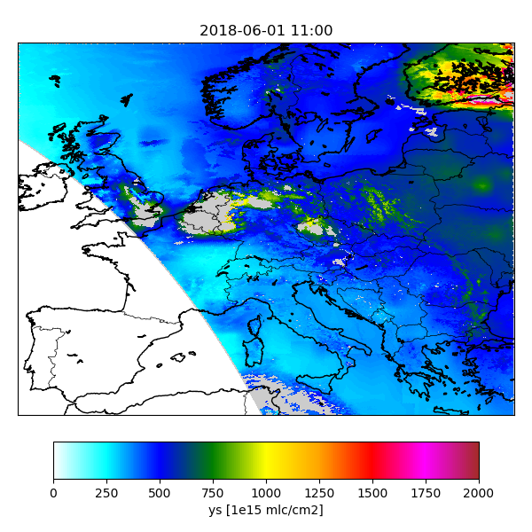
The configuration describes the time range for which plots are to be made. The names of the input files (output of the observation operator) should be specified for both the data and the state files:

cso.tutorial.sim-catalogue.input.data.file        :  ${my.work}/CSO-oper/CSO_output_%Y%m%d_%H%M_data.nc
cso.tutorial.sim-catalogue.input.state.file       :  ${my.work}/CSO-oper/CSO_output_%Y%m%d_%H%M_state.nc

The variables for which plots should be made are specified as a list of keywords; the current settings specify that figures should be for the retrieval yr and for the simulation ys:

cso.tutorial.sim-catalogue.vars                   :  yr ys

For these variables it is necessary to define whether they should be read from a variable in the data or in the state file; this is done using the source specification:

cso.tutorial.sim-catalogue.var.yr.source          :  data:yr

cso.tutorial.sim-catalogue.var.ys.source          :  state:ys

The names of the created figures is composed from the base name of the converted files and the variable that is plotted:

/work/yourname/CSO-Tests/CSO-oper/sim-catalogue/2018/06/01/S5p_RPRO_NO2_20180601_1100_yr.png
                                                           S5p_RPRO_NO2_20180601_1100_ys.png
                                                           :

Index pages are created to facilitate browsing through the figures. The index is created with the index task of the job. As shown above, the work is done by the Indexer class that can be accessed from the utopya module. The arguments that initialize the class specify the name of an rcfile with settings (tutorial-s5p.rc) and that the settings start with keywords 'cso.tutorial.sim-catalogue-index'.

When successful, the index creator displays an url that could be loaded in a browser:

Browse to:
  file:///work/yourname/CSO-Tests/CSO-oper/sim-catalogue/index.html

Step 8 - Demo with MPI parallel domain decomposition¶

The observation operator code supports MPI-parallel domain decomposition. Local domain will only simulate observations that overlap with the local domain; on output, the simulations from all domains are gathered and written out.

By default the observation operator code does not assume that it is running under MPI. The MPI related parts of the code are enabled only if the _MPI macro is defined. For example, the following lines are used in cso_comm.F90 to switch between an MPI and a serial code:

#ifdef _MPI
    ! collect from all pe and broadcast result:
    call MPI_Gather( value, 1, MPI_DTYPE, values, 1, MPI_DTYPE, self%root_id, self%comm, ierror=status )
    IF_MPI_NOT_OK_RETURN(status=1)
#else
    ! copy:
    values = value
#endif

To enable the MPI environment, edit the cso.inc macro include file and define the special macro:

! define macro's:
#define _MPI

Remove existing object files, and compile the executable:

cd src
make clean
make tutorial_oper_S5p.x
cd ..

An MPI job that creates 4 sub domains is probably started using:

mpirun -n 4 src/tutorial_oper_S5p.x

See the manuals of your MPI environment for fine tuning. It is for example useful to have the output messages per sub domain written to a different file, or to have every line preceded by the processor id.

Check the messages from the sub-domains to see if the decomposition worked correctly; for the first domain, the output should inclule:

Tutorial: global domain             : [  -10.00,   30.00] x [   35.00,   65.00]
Tutorial: number of processors      : 4
Tutorial: processor id (0-based)    : 0
Tutorial: decompostion              : 2 x 2
Tutorial: domain id (0-based)       : 0 , 0
Tutorial: local domain              : [  -10.00,   10.00] x [   35.00,   50.00]

The output of the domain-decomposition should be the same as for the serial code, which could be checked using the catalogue.

Step 9 - Gridded averages¶

(See Gridding chapter for main description)

The cso.tutorial.gridded job is configured in rc/tutorial.rc to create gridded averages of retrievals and/or simulations.

The input for this job should include the footprint information, for example the converted files:

S5p_RPRO_NO2_03272.nc
S5p_RPRO_NO2_03273.nc
:

or the output from the observation operator:

CSO_output_20180601_0300_data.nc
CSO_output_20180601_0300_state.nc
CSO_output_20180601_0500_data.nc
CSO_output_20180601_0500_state.nc
:

The result is a set of files with gridded averages:

S5p_RPRO_NO2_03272.nc
S5p_RPRO_NO2_03273.nc
:

or:

CSO_output_20180601_0300_gridded.nc
CSO_output_20180601_0500_gridded.nc
:

The configuration of the gridding job is:

! single step:
cso.tutorial.gridded.class        :  utopya.UtopyaJobStep
! catalogue creation task:
cso.tutorial.gridded.task.class   :  cso.CSO_GriddedAverage
cso.tutorial.gridded.task.args    :  '${PWD}/config/tutorial/tutorial-s5p.rc', \
                                      rcbase='cso.tutorial.gridded'

It is also possible to create a catalogue of the gridded fields.

The gridded fields have a time dimension, and therefore a temporal average could be produced using the NCO tools:

ncra  CSO_output_20180601_??00_gridded.nc  CSO_output_20180601_aver_gridded.nc

The figure shows an example of averaged NO2 retrievals.

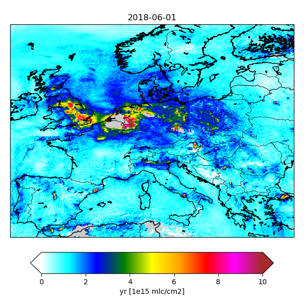
Daily averaged gridded S5p NO2 columns — *Gridded S5p NO2 columns averaged over a day.*¶

Step 10 - Update documentation¶

The documentation is generated from files included in the CSO tree. See the Documentation chapter for the format of the documentation source.

By now you must have found many missing items and errata in the documentation. Feel free to correct them, and (re)create the documentation using:

make docu

To remove temporary files, use:

make clean