Observation operator

This chapter describes the Fortran code with the satellite observation operator.

The observation operator code consists of Fortran files that should be added to a simulation model. For testing, a dummy program is provided that reads orbit files created by the preprocessor, simulates a (fake) concentration profile, convolves this with the averaging kernels, and writes this to a file as a simulated retrieval.

Retrieval simulation equations

A retrieval product is denoted with:

\[\mathbf{y}_r\]

The product is assumed to be a profile defined on \(n_r\) layers, which could be one in case of a total column.

The simulation of a retrieval product from a model state is denoted with:

\[\mathbf{y}_s ~=~ \mathbf{y}_{a} ~+~ \mathbf{A}\ \left(\ \mathbf{x}_s\ -\ \mathbf{x}_a\ \right)\]

where:

• \(\mathbf{x}_a\) is an a priori profile used by the retrieval algorithm, defined on \(n_a\) layers;

• \(\mathbf{y}_{a}\) is the retrieved a priori profile defeined on the \(n_r\) retreival layers; this is simply equal to \(\mathbf{x}_a\) in case \(n_r=n_a\), or a vertical integration of \(\mathbf{x}_a\) in case \(n_r<n_a\);

• \(\mathbf{x}_s\) is the simulated profiles derived from the model state, defined on the same \(n_a\) layers as \(\mathbf{x}_a\) and having the same units;

• \(\mathbf{A}\) is the averaging kernel matrix with shape \((n_r,n_a)\);

• \(\mathbf{y}_s\) is the simulated retrieval.

In some satellite products there is no a priori profile, or it is implicitly defined to be zero; in that case, both \(\mathbf{x}_a\) and \(\mathbf{y}_{a}\) are omitted.

The simulated profile \(\mathbf{x}_s\) is assumed to be derived from a model state using:

\[\mathbf{x}_s ~=~ \mathbf{V}\ \mathbf{G}\ \bar{\mathbf{c}}\]

where:

• \(\bar{\mathbf{c}}\) is the model state, which probably consists of a 3D array of concentrations;

• \(\mathbf{G}\) extracts a simulated profile from the state using horizontal interplation; the result is defined on the original model layers;

• \(\mathbf{V}\) applies a vertical remapping or interpolation; the result should be valid for the same layers as the a priori profile \(\mathbf{y}_a\) and also have the same units;

The simulation equation is often sumarized by combining the operators for the horizontal and vertical mapping and the kernel application:

\[\mathbf{H} ~=~ \mathbf{A}\ \mathbf{V}\ \mathbf{G}\]

which leads to:

\[\mathbf{y}_s ~=~ \left(\mathbf{y}_a-\mathbf{A}\mathbf{x}_a\right) ~+~ \mathbf{H}\ \bar{\mathbf{c}}\]

The convolution with the averaging kernel could also be applied to the true profile \(\mathbf{x}_t\) (defined at the a priori layers), which is the unknown but existing profile that is actually present in the observed atmosphere:

\[\mathbf{y}_t ~=~ \mathbf{y}_{a} ~+~ \mathbf{A}\ \left(\ \mathbf{x}_t\ -\ \mathbf{x}_a\ \right)\]

The following relation between the actual retrieval product and true retrieval is assumed:

\[\mathbf{y}_r ~-~ \mathbf{y}_t ~\sim~ \mathcal{N}\left(\mathbf{o},\mathbf{R}\right)\]

where:

• \(\mathbf{R}\) is the \((n_r,n_r)\) retrieval error covariance.

Notations

This table summarizes the entities used in the above and following equations.

The ‘varname’ columns refer to the names used in the tutorial and template configurations, and therefore also in the data files. The variables are user-defined and could be changed if needed.

Size \(n_p\) is the number of pixels, size \(n_z\) is the number of layers in the model.

shape	simulation			gradient
	entitie	varname	description	entitie	varname
\((n_x,n_y,n_z)\)	\(\bar{\mathbf{c}}\)		model concentrations	\(\bar{\mathbf{g}}\)
\((n_x,n_y,n_z+1)\)	\(\bar{\mathbf{p}}\)		model half-level pressures
	\(\mathbf{G}\)		mapping operator to footprints	\(\mathbf{G}^T\)
\((n_z,n_p)\)	\(\mathbf{c}\)	mod_conc	model concentration profile	\(\mathbf{g}\)	mod_g
\((n_z+1,n_p)\)	\(\mathbf{p}\)	mod_hp	model half-level pressure profile
	\(\mathbf{V}\)		mapping operator to apriori layers	\(\mathbf{V}^T\)
\((n_a,n_p)\)	\(\mathbf{x_a}\)	xa	a priori profile
	\(\mathbf{x_s}\)	xs	simulated profile	\(\mathbf{f}\)	f
	\(\mathbf{x_t}\)		true profile
\((n_a+1,n_p)\)	\(\mathbf{p_a}\)	hp	a priori half-level pressure profile
\((n_r,n_a,n_p)\)	\(\mathbf{A}\)	A	averaging kernel	\(\mathbf{A}^T\)
\((n_r,n_p)\)	\(\mathbf{y_a}\)	ya	a priori retrieved profile
	\(\mathbf{y_s}\)	ys	simulated retrieved profile	\(\mathbf{\epsilon}\)	eps
	\(\mathbf{y_r}\)	yr	retrieved profile
	\(\mathbf{y_t}\)		true retrieved profile
\((n_r+1,n_p)\)	\(\mathbf{p_r}\)	hpr	retrieval half-level pressure profile
\((n_r,n_r,n_p)\)	\(\mathbf{R}\)	vr (diag)	retrieval error covariance

Requirements

The source code of the observation operator requires that the following is available:

• recent Fortran compiler with support for F2008 constructs (for example GFortran v8.2.0)

• netCDF library

• eventually an MPI wrapper

Source code overview

The demo code is included in the subdirectory:

oper/src/Makefile
         Makefile_config_template
         cso.F90
         cso.inc
         cso_comm.F90
         :
         cso_tools.F90
         tutorial_oper_S5p.F90
     tutorial.rc

Compiling and running tutorial

For testing, copy the entire sub directory to a work directory; configuration assumes a location in the work directory of the pre-processor where the converted orbit files are:

cd /work/yourname/CSO-Tests
cp -r /home/yourname/CSO/oper CSO-oper

Go into it:

cd CSO-oper

To compile the code, the following should be used:

cd src/
make tutorial_oper_S5p.x
cd ..

This will probably fail because of incorrect compiler and library settings. Create a copy of the Makefile settings for your own machine, and edit where needed:

cd src
cp Makefile_config_template  Makefile_config_inst-mach

Ensure that that Makefile includes the new settings:

include Makefile_config_inst-mach

If with this settings the executable has been compiled successful, run it using:

./src/tutorial_oper_S5p.x

The follow sections show step by step the elements of observation operator code.

Initialization

All entities of the CSO code are accessible via the top-level CSO module:

use CSO, only : T_CSO
use CSO, only : T_CSO_RcFile
:

As convention, all CSO specific types have a name with prefix T_CSO_. The types define Fortran2008 classes with their methods attached.

A main object for the CSO module should be declared, and initalized/cleared at the start/end of the program:

! main object for CSO data:
type(T_CSO)                   ::  csod

! return status:
integer                       ::  status

! init CSO data:
call csod%Init( status )
if (status/=0) stop

:

! done with CSO:
call csod%Done( status )
if (status/=0) stop

Each method has an integer status output argument, which will be zero if everything is ok, and positive in case of an error. In some lower-level routines the status could be negative to indicate a warning.

See the MPI parallel code section for initialization in an MPI-parallel program.

Logging

By default the messages from the operator are written to standard output.

The main object has a method that could be used to reset the destination to a file unit used by the main program:

integer       ::  logfu

! log file unit:
logfu = 123
! open logfile:
open( unit=logfu, file='tutorial.out', status='replace' )

! also write CSO messages to this unit:
call csod%SetLogging( status, unit=logfu )
if (status/=0) stop

Alternative, the operator could be configured to write messages to a seperate file:

! redirect messages:
call csod%SetLogging( status, file='cso.log' )
if (status/=0) stop

In an MPI parallel program, the writing of messages could also be limitted to the root processor only:

! limit messages ...
call csod%SetLogging( status, root_only=.true. )
if (status/=0) stop

MPI parallel code

The observation operator code supports MPI-parallel domain decomposition. A local domain will only (partly) simulate observations that overlap (partly) with the local domain; on output, the simulations from all domains are gathered and written.

By default the observation operator code does not assume that it is running under MPI. The MPI related parts of the code are enabled only if the _MPI macro is defined. For example, the following lines are used in cso_comm.F90 to switch between an MPI and a serial code:

#ifdef _MPI
    ! collect from all pe and broadcast result:
    call MPI_Gather( value, 1, MPI_DTYPE, values, 1, MPI_DTYPE, self%root_id, self%comm, ierror=status )
    IF_MPI_NOT_OK_RETURN(status=1)
#else
    ! copy:
    values = value
#endif

To enable the MPI environment, edit the cso.inc macro include file and define the special macro:

! define macro's:
#define _MPI

Ensure that the cso*.F90 are re-compiled again after changing the macro definition.

The CSO operator code should be initialized using the MPI communicator in this case. For a main program with Fortran2008 MPI types (as the tutorial), the initialization should look like:

use MPI_F08, only : MPI_Comm
use MPI_F08, only : MPI_COMM_WORLD

! communicator:
type(MPI_Comm)                ::  comm

! main object for CSO data:
type(T_CSO)                   ::  csod

...

! use global communicator:
comm = MPI_COMM_WORLD

! init CSO module including MPI communication:
call csod%Init( status, comm=comm )
if (status/=0) stop

For main programs using integer MPI handles, use:

include 'mpi.h'

! communicator:
integer                       ::  icomm

...

! use global communicator:
icomm = MPI_COMM_WORLD

! init CSO module including MPI communication:
call csod%Init( status, icomm=icomm )
if (status/=0) stop

An MPI job that creates 4 sub domains is probably started using:

mpirun -n 4 src/tutorial_oper_S5p.x

See the manuals of your MPI environment for details. It is for example useful to have the output messages per sub domain written to a different file, or to have every line preceded by the processor id.

Check the messages from the sub-domains to see if the decomposition worked correctly; for the first domain, the output should inclule:

Tutorial: global domain             : [  -10.00,   30.00] x [   35.00,   65.00]
Tutorial: number of processors      : 4
Tutorial: processor id (0-based)    : 0
Tutorial: decompostion              : 2 x 2
Tutorial: domain id (0-based)       : 0 , 0
Tutorial: local domain              : [  -10.00,   10.00] x [   35.00,   50.00]

The output of the domain-decomposition should be the same as for the serial code.

Settings for test program

The main program tutorial_oper_S5p.F90 reads settings from the file:

tutorial.rc

The following code is used to initialize and clear an ojbect that is used to read the settings:

type(T_CSO_RcFile)            ::  rcf

! read:
call rcf%Init( 'tutorial.rc', status )
if (status/=0) stop

...

! done with settings:
call rcf%Done( status )
if (status/=0) stop

Settings are read using the keyword, for example:

! get name of listing file:
call rcf%Get( 'tutorial.S5p.no2.listing', listing_filename, status )
if (status/=0) stop

Some of the settings are only needed by the main program, and define a time loop and an assumed simulation domain:

! time range:
tutorial.timerange.start           :  2018-06-01 00:00
tutorial.timerange.end             :  2018-06-02 00:00

! selected domain:
tutorial.domain.west               :  -10
tutorial.domain.east               :   30
tutorial.domain.south              :   35
tutorial.domain.north              :   65

Other settings are needed by the observation operator code and these are described in the following sections.

Listing file

The program will perform a time loop with hourly steps. At selected times, orbits are selected for which the average time falls within an interval. The orbits are selected using a listing file that has been created by the pre-processing, as described for example in the NO₂ Listing file section.

The (relative) location of the listing file with orbit file names and time ranges should be specified in the rcfile:

! listing file for converted NO2 product:
tutorial.S5p.no2.listing           : ../S5p/RPRO/NO2/CAMS/listing.csv

In the program, the name of the listing file is first read from the settings; a listing object is created given this filename:

use CSO, only : T_CSO_Listing

character(len=1024)           ::  listing_filename
type(T_CSO_Listing)           ::  listing

! listing file:
call rcf%Get( trim(rcbase)//'.listing', listing_filename, status )
if (status/=0) stop

! read listing file:
call listing%Init( listing_filename, status )
if (status/=0) stop

...

! done with listing:
call listing%Done( status )
if (status/=0) stop

To search for all oribits with an average time within a specific hour, use the date/time objects from CSO:

use CSO, only : T_CSO_DateTime, CSO_DateTime

type(T_CSO_DateTime)          ::  t1, t2
character(len=1024)           ::  orbit_filename

! hour range:
t1 = CSO_DateTime( year=2018, month=6, day=1, hour=10, min=0 )
t2 = CSO_DateTime( year=2018, month=6, day=1, hour=11, min=0 )

! get name of file for orbit time average within [t1,t2]:
call listing%SearchFile( t1, t2, 'aver', orbit_filename, status )
if (status/=0) stop

! found?
if ( len_trim(orbit_filename) > 0 ) then

  ...

end if

The tutorial progam actually reads a start and end time and performs a loop over hours, see the code for this implementation.

Satellite data

When an orbit file is found for the requested time interval, a data object should be defined to read the content. The data object contains a copy of the original input, but limited to the model domain that might be smaller than domain extracted from the original orbits. The following entities are included:

• footprints of selected pixels (longitudes, latitudes)

• footprints of original track;

• pressure profiles;

• averaging kernels;

• retrieved values;

• retrieval variance;

• optional: horizontal mapping information.

The data object is used to creaste a state object with the simulation. The state contains:

• optional: original model concentration and pressure profiles;

• optional: concentration profile at a priori layers;

• simulated retrieval.

In an ensemble application, one data object might be defined and multiple state objects, one for each ensemble member.

Data object

Initialize an orbit data object using the name of the data file. The object also requires settings from the rcfile, therefore pass the rcfile object and the base keyword too:

use CSO, only : T_CSO_Sat_Data

! orbit data:
type(T_CSO_Sat_Data)          ::  sdata

! inititalize orbit data,
! read all footprints available in file:
call sdata%Init( rcF, 'tutorial.S5p.no2', orbit_filename, status )
if (status/=0) stop

...

! done with state:
call sstate%Done( sdata, status )
if (status/=0) stop

The operator needs some specific information to know which data should be read. For example, tell it to read information on the original tracks too; this will be saved in the output to facilitate creation of map plots:

! also read info on original track (T|F)?
! if enabled, this will be stored in the output too:
tutorial.S5p.no2.with_track        :  T

Pixel selection

The initialization will only read the footprints. All footprints in the file are read, thus also the footprints outside the model domain (or the local domain in case of domain decomposition). The next step is to select only those pixels that should be simulated at least partly from the (local) domain. This could for example be done using only the footprint center, which in a domain-decomposition has the advantage that a pixel is simulated from only one sub-domain. More accurate is to simulate an average over the footprint area, as described in the Horizontal mapping section; in case of domain decomposition, multiple local domains might then contribute to the simulation of a single pixel. The code should flag all pixels that should be simulated using information from the local domain:

integer                       ::  nglb
real, pointer                 ::  glb_lon(:)       ! (nglb)
real, pointer                 ::  glb_lat(:)       ! (nglb)
real, pointer                 ::  glb_clons(:,:)   ! (nglb,4)
real, pointer                 ::  glb_clats(:,:)   ! (nglb,4)
logical, pointer              ::  glb_select(:)    ! (nglb)
integer                       ::  iglb

! obtain from the orbit:
! - number of footprints (global, all pixels in file)
! - pointers to arrays with footprint centers  (not used here!)
! - pointers to arrays with footprint corners
! - pointer to to selection flags, should be used to select pixels overlapping with local domain
call sdata%Get( status, nglb=nglb, &
                         glb_lon=glb_lon, glb_lat=glb_lat, &
                         glb_clons=glb_clons, glb_clats=glb_clats, &
                         glb_select=glb_select )
if (status/=0) stop

! select pixels that overlap with local domain;
! loop over global pixels:
do iglb = 1, nglb
  !!~ decide if pixel center is part of local domain:
  !glb_select(iglb) = (glb_lon(iglb) >= dom_west ) .and. (glb_lon(iglb) <= dom_east ) .and. &
  !                   (glb_lat(iglb) >= dom_south) .and. (glb_lat(iglb) <= dom_north)
  !~ check if footprint overlaps (partly) with domain,
  !  and if it is entirely in global domain;
  !  use bounding box of footprint to check:
  glb_select(iglb) = (maxval(glb_clons(:,iglb)) >= dom_west ) .and. (minval(glb_clons(:,iglb)) <= dom_east ) .and. &
                     (maxval(glb_clats(:,iglb)) >= dom_south) .and. (minval(glb_clats(:,iglb)) <= dom_north) .and. &
                     (minval(glb_clons(:,iglb)) >=     west ) .and. (maxval(glb_clons(:,iglb)) <=     east ) .and. &
                     (minval(glb_clats(:,iglb)) >=     south) .and. (maxval(glb_clats(:,iglb)) <=     north)
end do ! iglb

The selection flags are stored in an internal array in the satellite data object.

Reading selected pixels

Now that the pixel selection flags have been set, use the following call to read the retrieval data for the pixels selected for the local domain:

! read orbit, locally store only pixels that are flagged in 'glb_select'
! as having overplap with this domain:
call sdata%Read( status )
if (status/=0) stop

The operator should read variables from the data files that are needed to simulate a retrieval from the model arrays. This includes for example the pressures that define the a priori layers, the averaging kernel, and for this product, the airmass factor and tropopause level. Which variables should be read should defined in the settings using a list of names:

! data variables:
tutorial.S5p.no2.dvars             :  hp yr vr A M nla

For each of these, define the following detailed settings:

• A list of dimension names that define the shape of the data per pixel; these are used to allocate the correct storage and check the input; supported dimensions are:

  • layer and layeri for the a priori layers and layer interfaces;

  • retr for the retrieval layers

• The name of the source variables; these are the names used in the conversion step.

Example settings:

! half-level pressures:
!~ dimensions, copied from data file:
tutorial.S5p.no2.dvar.hp.dims      :  layeri
!~ source variable:
tutorial.S5p.no2.dvar.hp.source    :  pressure

! retrieval:
!~ dimensions, copied from data file:
tutorial.S5p.no2.dvar.yr.dims      :  retr
!~ source variable:
tutorial.S5p.no2.dvar.yr.source    :  vcd

! retrieval error covariance:
!~ dimensions, copied from data file:
tutorial.S5p.no2.dvar.vr.dims      :  retr retr
!~ source variable:
tutorial.S5p.no2.dvar.vr.source    :  vcd_errvar

! kernel:
!~ dimensions, copied from data file:
tutorial.S5p.no2.dvar.A.dims       :  retr layer
!~ source variable:
tutorial.S5p.no2.dvar.A.source     :  kernel_trop

! tropospheric airmass factor
!~ dimensions, copied from data file:
tutorial.S5p.no2.dvar.M.dims       :  retr
!~ source variable:
tutorial.S5p.no2.dvar.M.source     :  amf_trop

! number of apriori layers in retrieval layer:
!~ dimensions, copied from data file:
tutorial.S5p.no2.dvar.nla.dims     :  retr
!~ source variable:
tutorial.S5p.no2.dvar.nla.source   :  nla

After reading, the number of pixels in the local domain could be obtained with:

! obtain info on track: ! - number of local pixels call sdata%Get( status, npix=npix ) if (status/=0) stop

Simulation state definition

Simulated pixels will be stored in a state object. The state object will contain at least the simulated retrievals, but could also contain other simulated data at pixel locations.

State object

Declare, initialize, and clear a state object using:

use CSO, only : T_CSO_Sat_State

type(T_CSO_Sat_State)         ::  sstate

!
! initialize simulation state using the satellite data object;
! optional arguments:
!   description='long name'    : used for output attributes
call sstate%Init( sdata, rcF, rcbase, status, &
                     description='simulated retrievals' )
if (status/=0) stop

...

! done with state:
call sstate%Done( sdata, status )
if (status/=0) stop

A list of names for the variables to be defined in the state is read from the settings:

! state varaiables to be put out from model:
tutorial.S5p.no2.vars    :  mod_conc mod_hp mod_tcc mod_cc hx ys Sy M_m A_m yr_m ys_m

For each of these variables, define detailed settings on how to create them. Two methods are currently possible:

• The model should fill the variables from its own arrays, e.g. model concentrations and pressures.

• Variables are computed from each other using a predefined formula, for exmaple for a kernel convolution.

The following sub-sections define the details of the variable definition; the actual creation is defined in the sections Horizontal mapping and Formula application.

Dimension definition

For each variable, a list of dimension names should be specified to know it the variable is (per pixel) a scalar, a profile, or a matrix. For example, the total cloud cover in the model is a scalar and does not require a dimension definition:

! total cloud cover:
!~ no extra dimensions:
tutorial.S5p.no2.var.mod_tcc.dims             :

But the model concentrations are defined at the model layers, and therefore this should be a dimension:

! model concentration profile:
!~ model layer dimension:
tutorial.S5p.no2.var.mod_conc.dims            :  model_layer

Two types of dimension names are supported:

• Dimensions from the data files, for example:

  • layer and layeri for the a priori layers and layer interfaces;

  • retr for the retrieval layers

• Other dimension names, that should be defined by the user.

After reading the settings, the user should inquire the state object for the dimension names thtat should be defined, and assign the correct length. This is done using the following code:

! user defined dimensions:
integer                           ::  nudim
integer                           ::  iudim
character(len=32)                 ::  udimname

...

! number of user defined dimensions:
call sstate%Get( status, nudim=nudim )
if (status/=0) stop
! loop:
do iudim = 1, nudim
  ! get dimension name to be defined:
  call sstate%GetDim( iudim, status, name=udimname )
  if (status/=0) stop
  ! switch:
  select case ( trim(udimname) )
    !~ model layers:
    case ( 'model_layer' )
      ! define:
      call sstate%SetDim( udimname, nz, status )
      if (status/=0) stop
    !~ model layer interfaces:
    case ( 'model_layeri' )
      ! define:
      call sstate%SetDim( udimname, nz+1, status )
      if (status/=0) stop
    !~ unknown ...
    case default
      write (*,'("unsupported dimension `",a,"`")') trim(udimname)
      TRACEBACK; status=1; call Exit(status)
  end select
end do ! idim

When all dimension are defined, the arrays in the state could be allocated. This is done by the following call:

! dimension defined, allocate storage: call sstate%EndDef( status ) if (status/=0) stop

Variable attributes

The state variables should be accompanied with attributes. At least a units and a long_name or standard_name should be defined.

Attributes are defined using a list of attribute names, and for each an assignment:

!~ standard attributes:
tutorial.S5p.no2.var.mod_conc.attrs           :  long_name units
tutorial.S5p.no2.var.mod_conc.attr.long_name  :  model NO2 concentrations
tutorial.S5p.no2.var.mod_conc.attr.units      :  ppb

Horizontal mapping

In the simulation equations the mapping from model grid cells to satellite footprint is denoted by the operator:

\[\mathbf{c} ~=~ \mathbf{G}\ \bar{\mathbf{c}}\]

where:

• \(\bar{\mathbf{c}}\) is the model state (3D grid);

• \(\mathbf{x}\) a profile over a pixel footprint, defined on the model layers.

We assume that the horizontal averaging over the footprint is the same for each model layer, so \(\textbf{G}\) is acutally an operator on a 2D field that is applied repeatively.

How the horizontal mapping is done depends strongly on the simulation grid. It should therefore be handled by the user. For convenience, a sample code is available to average concentrentrations on a reguler grid over the area of a footprint. The result is computed as a weighted average over grid cells:

\[\mathbf{G}_p\ \bar{\mathbf{c}}(:,:) ~=~ \left(\ \sum\limits_{k\in K_p} \bar{c}(i_k,j_k)\ w_{p,k}\ \right)/w_p\]

where the weights represent area in m²:

• \(w_p\) is the footprint area of pixel \(p\);

• \(w_{p,k}\) is the fraction of this area that overlaps with the cell \((i_k,j_k)\).

The set \(K_p\) holds the factioning of pixel \(p\).

The figure below illustrates how the weights \(w_k\) are determined. A footprint is devided into triangles, and the centroids are collected as sample points. For each centroid, an originating model grid cell is chosen, in the tutorial code this is simply the model grid cell holding the centroid. The weight of each grid cell in the footprint average is then defined as the fraction of the area covered by the triangles for the centroids has been assigned to the grid cell.

The division in triangles is done recursively up to level defined by the user. Level 0 means no division, and the only centroid is the center of the footprint. Level 1 means as single division into triangles, leading to 4 centroids. With level 2, the first 4 triangles are devided into 4 new triangles, leading to 16 centroids in total; similar, level 3 will lead to 64 centroids.

The level number that is needed depends on ratio between footprint size and grid cell size; if the footprints are rather large compared to the model, then a higher level is needed. For the tutorial code, the level is defined in the settings with:

! recursion level for division of footprints into triangles:
tutorial.mapping.levels            :  3

This weights have been used to create the maps on the right in the figure below. The colors show the sum of the weights that are assigned to a cell during the mapping of the pixels. At the center of the orbit, this sum could reach values up to 6, which indicates that a grid cell is covered by about 6 rather small pixels. For level 0 the sums are rather noisy, but for higher recursion levels the pattern becomes more smooth.

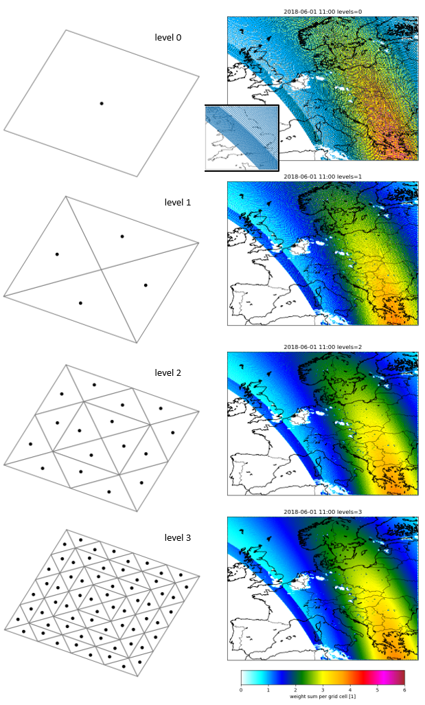
Illustration of mapping from grid cells to footprints. Left column shows distribution of (triangle) in 4-sided footprint for different levels of triangularization. Maps on the right show total weight of grid cells in demo configuration in mapping to S5p orbit. The small figure shows the centers of S5p pixels, which are closer to each other at the edges of the swath.

The CSO code contains a class to perform mapping from a regular grid to footprint area. Initialize the mapping operator using a grid description:

use CSO, only : T_CSO_GridMapping

type(T_CSO_GridMapping)       ::  GridMapping
integer                       ::  mapping_levels

...

! mapping level:
mapping_levels = 3

! init grid mapping using:
! - west and south bound of global(!) grid;
! - grid spacing;
! - local grid cell offset in global grid;
! - local grid shape
! - recursion level
call GridMapping%Init( west , dlon, dom_ilon0, nlon, &
                       south, dlat, dom_ilat0, nlat, &
                        mapping_levels, status )
if (status/=0) stop

...

! done with grid mapping:
call GridMapping%Done( status )
if (status/=0) stop

Assign pointers to the arrays holding the pixel corners:

! pixel footprints:
real, pointer                     ::  lons(:), lats(:)         ! (npix)
real, pointer                     ::  clons(:,:), clats(:,:)   ! (ncorner,npix)

...

! pointers to (*,pixel) arrays:
! - footprint centers  (not used, for inspiration ..)
! - footprint corners
call sdata%Get( status, lons=lons, lats=lats, clons=clons, clats=clats )
if (status/=0) stop

Pass these to the mapping object, which will in return set pointers to arrays that hold the indices of source cells and their weight in the footprint average:

integer, pointer              ::  ii(:), jj(:)
real, pointer                 ::  ww(:)
integer, pointer              ::  iw0(:), nw(:)

...

! get pointers to mapping arrays for all pixels:
! - areas(1:npix)            : pixel area [m2]
! - iw0(1:npix), nw(1:npix)  : offset and number of elements in ii/jj/ww
! - ii(:), jj(:), ww(:)      : cell and weight arrays for mapping to footprint,
call GridMapping%GetWeights( clons, clats, &
                               areas, iw0, nw, ii, jj, ww, status )
if (status/=0) stop

The number nw is the number of source cells in the local domain that contribute to the footprint average. This might be zero in case the pixel selection was quick-and-dirty (as in the tutorial), therefore it is necessary to check if it is at least 1.

Eventually store the indices and weights in the satellite data object so that they can be put out for later usage. In case of domain decomposition it is important to store the indices in the global grid to have unique values that can be used independent of the chosen decomposition:

! store mapping weights, might be saved and used to create gridded averages;
! cell indices ii/jj need to be the global index numbers!
call sdata%SetMapping( areas, nw, dom_ilon0+ii, dom_ilat0+jj, ww, status )
if (status/=0) stop

To have these actually put out, the following flag should be enabled in the settings:

! put out mapping arrays? used for regridding:
tutorial.S5p.no2.with_mapping      :  T

When the mapping arrays are stored in the data structure, they can be accessed again using pointers:

! pointers to mapping arrays:
integer, pointer               ::  nw(:)      ! (npix)
integer, pointer               ::  iw0(:)     ! (npix)
integer, pointer               ::  glb_ii(:)  ! (nmap)
integer, pointer               ::  glb_jj(:)  ! (nmap)
real, pointer                  ::  ww(:)      ! (nmap)
real, pointer                  ::  areas(:)   ! (npix)

! set pointers to mapping arrays;
! note that 'glb_ii' and 'glb_jj' point to global index values:
call sdata%Get( status, nw=nw, iw0=iw0, ii=glb_ii, jj=glb_jj, ww=ww, areas=areas )
if (status/=0) stop

This could be useful to simulate concentrations more than once, for example for a first guess state and for analysis.

User defined variables

The horizontal mapping information could now be used to extract model variables at pixel locations.

First obtain information on the number of user-defined variables, their names, and their units. Variables that should be formed by a formula are not part of this, they are filled later when all user-defined variables are available. Then perform a loop over the variables, and use a case selection per variable since each depends on different model data. In the code this looks like:

! user defined variables:
integer                           ::  nuvar
integer                           ::  iuvar
character(len=64), allocatable    ::  uvarnames(:)  ! (nuvar)
character(len=64), allocatable    ::  uvarunits(:)  ! (nuvar)

...

! number of user defined variables:
call sstate%Get( status, nuvar=nuvar )
if (status/=0) stop
! any user defined?
if ( nuvar > 0 ) then

  ! storage for variable names and units:
  allocate( uvarnames(nuvar), stat=status )
  if (status/=0) stop
  allocate( uvarunits(nuvar), stat=status )
  if (status/=0) stop
  ! fill:
  call sstate%Get( status, uvarnames=uvarnames, uvarunits=uvarunits )
  if (status/=0) stop

  ! loop over variables:
  do iuvar = 1, nuvar
    ! info ..
    write (*,'("user defined variable: ",a)') trim(uvarnames(iuvar))
    ! switch:
    select case ( trim(uvarnames(iuvar)) )

      !~ model concentrations
      case ( 'mod_conc' )
        ...

      !~ cloud cover: total:
      case ( 'mod_tcc' )
        ...

      !~
      case default
        write (*,'("unsupported variable name `",a,"`")') trim(uvarnames(iuvar))
        stop
    end select

  end do ! user defined variables

  ! info ...
  write (*,'("end ...")')

  ! clear:
  deallocate( uvarnames, stat=status )
  if (status/=0) stop
  deallocate( uvarunits, stat=status )
  if (status/=0) stop

For each case, specficic code should be implemented to extract values for the correct model arrays. It is useful to first check if the units in the model are the same as the target units specified in the settings (see Variable attributes section). Then obtain a pointer to the storage allocated for the simulation; depending on the specified dimensions, this could be a “0D” (scalar), “1D” (profile), or “2D” (matrix) array. Fill the array in a loop over the pixels, and using the grid cell indices and weights from the mapping. For the model concentrations this looks like:

! pixel arrays:
real, pointer                     ::  data0(:)          ! (npix)
real, pointer                     ::  data1(:,:)        ! (:,npix)

! pixel counter and index:
integer                           ::  npix
integer                           ::  ipix
! mapping index:
integer                           ::  iw

...

!~ model concentrations
case ( 'mod_conc' )
  ! check units:
  if ( trim(uvarunits(iuvar)) /= 'ppb' ) then
    write (*,'("variable `",a,"` requires conversion to `",a,"` from `",a,"`")') &
            trim(uvarnames(iuvar)), trim(uvarunits(iuvar)), 'ppb'
  end if
  ! get pointer to target array with shape (nz,npix):
  call sstate%GetData( status, name=uvarnames(iuvar), data1=data1 )
  if (status/=0) stop
  ! loop over pixels:
  do ipix = 1, npix
    ! any source contributions?
    if ( nw(ipix) > 0 ) then
      ! init sum:
      data1(:,ipix) = 0.0
      ! loop over source contributions:
      do iw = iw0(ipix)+1, iw0(ipix)+nw(ipix)
        ! add contribution:
        data1(:,ipix) = data1(:,ipix) + conc(ii(iw),jj(iw),:) * ww(iw)/areas(ipix)
      end do ! iw
    end if ! nw > 0
  end do ! ipix

Formula application

If a variable should be computed from other variables, define a formula.

A formula description consists of two lines, for example:

tutorial.S5p.no2.var.y.formula               :  LayerAverage( hp, mod_hp, mod_conc )
tutorial.S5p.no2.var.y.formula_terms         :  hp: hp mod_hp: mod_hp mod_conc: mod_conc

The formula line contains a description of the formula to be applied. This description is just a keyword, the parenthes and arguments in this example are interpreted. The formula_terms connect arguments of the formula to actual variables. The observation operator uses this to search the correct variables for the operation.

Since the formula might be applied to simulated retrievals, it is essential that each domain has the same simulation in case a pixel overlaps more than one domain. This is done using the following code:

! inquire info on pixels covering multiple domains,
! setup exchange parameters:
call sdata%SetupExchange( status )
if (status/=0) stop
! exchange simulations:
call sstate%Exchange( sdata, status )
if (status/=0) stop

After this the routine that applies the formula’s is called:

! apply formula: kernel convolution etc:
call sstate%ApplyFormulas( sdata, status )
if (status/=0) stop

The following formulas are currently implemented.

LayerAverage( hp, mod_hp, mod_conc )

This formula will map a (model) concentration profile to another (retrieval) profile. In the simulation equations this is the operator:

\[\mathbf{x} ~=~ \mathbf{V}\ \mathbf{c}\]

where:

• \(\mathbf{c}\) is a profile defined on model layers;

• \(\mathbf{x}\) is a profile defined on a priori layers.

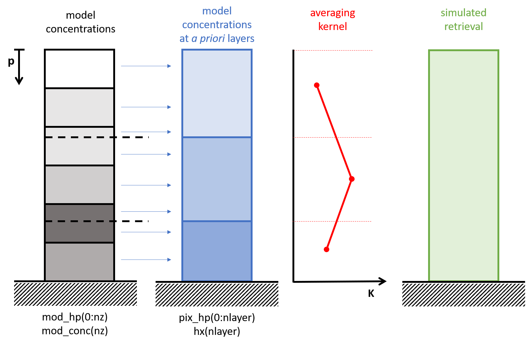
The figure illustrates all vertical layer definitions used in the satellite simulation; the operator \(\mathbf{V}\) is the first operation that converts from model layers to a priori layers.

For atmpospheric profiles the layer boundaries are typical pressures; the distribution in fraction will then conserve the air mass in the column. If the averaging kernel is defined for the entire atmosphere, the model profile needs to be defined up to a pressure of zero. If the model top is lower, at least one extra layer should be added to fill the remaining part of the atmosphere, for example holding a zero concentration.

Before the pressure layers of the model could be mapped to the target pressure layers, the surface pressures are be alligned. If the cocentration units are mass mixing ratio’s (kg tracer per kg air), this scaling will slightly change the total tracer mass. If this is problematic, the concentrations should first be converted to something equivalent to kg tracer per layer.

The mapping fractions from model layers to a priori layers are computed given the (aligned) pressure profiles. The fractions are computed independend of the directions of the profiles: both could be either bottom-up or top-down, and in direction differ from eachother.

The units of the source and target profile are compared to decide on the correct mapping. The user might need to implement additional unit conversions if needed. Different weighting methods are used depending on the conversion:

• assign a sum of source fractions:

  \[x_j ~=~ \sum\limits_{i}\ c_i\ w_{ij}\]

  with \(w_{ij}\) the faction of source interval \(i\) that overlaps with target interval \(j\);

• assign a sum of source fractions weighted with the source pressure change:

  \[x_j ~=~ \sum\limits_{i}\ c_i\ \mbox{d}p_i\ w_{ij}\]

  with \(w_{ij}\) the faction of source interval \(i\) with pressure change \(\mbox{d}p_i\) that overlaps with target interval \(j\);

• assign a sum of source fractions weighted with the source pressure change and normalized with the destination pressure change:

  \[x_j ~=~ \sum\limits_{i}\ c_i\ \mbox{d}p_i\ w_{ij}\ /\ \mbox{d}p_j\]

  with \(w_{ij}\) the faction of source interval \(i\) with pressure change \(\mbox{d}p_i\) that overlaps with target interval \(j\) with pressure change \(\mbox{d}p_j\).

The arguments to the formula are:

• hp : interface pressures for target profile;

• mod_hp : interface pressures for source profile;

• mod_conc : concentration profile

Example usage:

! model concentrations at apriori layers:
!~ apriori layers:
tutorial.S5p.no2.var.xs.dims                  :  layer
!~ how computed:
tutorial.S5p.no2.var.xs.formula               :  LayerAverage( hp, mod_hp, mod_conc )
tutorial.S5p.no2.var.xs.formula_terms         :  hp: hp mod_hp: mod_hp mod_conc: mod_conc

LayerAverageAdj( mod_hp, hp, f )

This formula denotes the transposed application of the vertical averaging as needed for variational assimilation (see Gradient computation):

\[\mathbf{g} ~=~ \mathbf{V}^T\ \mathbf{f}\]

Based on the units, the adjoint operation is for example (see the description of the LayerAverage formula):

\[g_{i} ~=~ \sum\limits_{j}\ f_j\ w_{ij}\]

with \(w_{ij}\) the faction of model interval \(i\) that overlaps with a priori interval \(j\).

Arguments are:

• mod_hp : interface pressures for model profile;

• hp : interface pressures for a priori profile;

• f : foring profile defined at a priori layers, probably created by ‘A^T eps’ formula.

Example usage:

!~ model layers:
tutorial.S5p.no2.var.mod_g.dims               :  model_layer
!~ how computed:
tutorial.S5p.no2.var.mod_g.formula            :  LayerAverageAdj( mod_hp, hp, f )
tutorial.S5p.no2.var.mod_g.formula_terms      :  mod_hp: mod_hp hp: hp f: f

A x

This formula denotes application of the averaging kernel:

\[\mathbf{y} ~=~ \mathbf{A}\ \mathbf{x}\]

Arguments are:

• A : averaging kernel

• x : (simulated) profile at a priori layers

Example usage:

! simulated retrievals
!~ retrieval layers:
tutorial.S5p.no2.var.ys.dims                  :  retr
!~ how computed:
tutorial.S5p.no2.var.ys.formula               :  A x
tutorial.S5p.no2.var.ys.formula_terms         :  A: A x: xs

A^T eps

This formula denotes application of the transposed averaging kernel to a forcing (see Gradient computation):

\[\mathbf{f} ~=~ \mathbf{A}^{T}\ \mathbf{\epsilon}\]

Arguments are:

• A : averaging kernel

• epsilon : simulation forcing at retrieval layers, probalby created by ‘R^{-1} ( ys - y )’ formula.

Example usage:

!~ apriori layers:
tutorial.S5p.no2.var.f.dims                  :  layer
!~ how computed:
tutorial.S5p.no2.var.f.formula               :  A^T eps
tutorial.S5p.no2.var.f.formula_terms         :  A: A eps: eps

PartialColumns( nla, x )

This formula could be used to create partial columns from a profile, as used for the NO₂ airmass factor correction (see section Averaging kernels):

\[\mathbf{Sx} ~=~ \sum_{l=1}^{n_{la}} (\mathbf{x})_l\]

Arguments are:

• nla : number of a priori layers to be combined in partial column

• x : (simulated) profile at a priori layers

Example usage:

! partial columns as sum over apriori layers
!~ retrieval layers:
tutorial.S5p.no2.var.Sx.dims                 :  retr
!~ how computed:
tutorial.S5p.no2.var.Sx.formula              :  PartialColumns( nla, x )
tutorial.S5p.no2.var.Sx.formula_terms        :  nla: nla x: xs

AltAirMassFactor( M, A, x, Sx )

Use this formula to compute a local airmass factor, as used for the NO₂ airmass factor correction (see section Averaging kernels):

\[\hat{M}^{trop}(\hat{\mathbf{x}}_a) ~=~ M^{trop} ~ \left(\mathbf{A}^{trop}\ \mathbf{x}_a\right) ~/~ \mathbf{Sx}\]

Arguments:

• M : tropospheric airmass factor from retieval product;

• A : original averaging kernel from retieval product;

• x : local concentration profile averaged over a priori layers;

• Sx : partial column of local profile, as computed by the ‘PartialColumns( nla, x )’ formula.

Example usage:

! airmass factor from local model
!~ retrieval layers:
tutorial.S5p.no2.var.M_m.dims                 :  retr
!~ how computed:
tutorial.S5p.no2.var.M_m.formula              :  AltAirMassFactor( M, A, x, Sx )
tutorial.S5p.no2.var.M_m.formula_terms        :  M: M A: A x: xs Sx: Sx

AltKernel( A, M, M_m )

Use this formula to compute an averaging kernel corrected with local airmass factor, as used for the NO₂ airmass factor correction (see section Averaging kernels):

\[\hat{\mathbf{A}}^{trop}(\hat{\mathbf{x}}_a) ~=~ \frac{M^{trop}}{\hat{M}^{trop}(\hat{\mathbf{x}}_a)}\ \mathbf{A}^{trop}\]

Arguments:

• A : original averaging kernel from retieval product

• M : tropospheric airmass factor from retieval product

• M_m : local airmass factor, computed using ‘AltAirMassFactor( M, A, x, Sx )’ formula

Example usage:

! kernel using airmass factor from local model
!~ retrieval layers times apriori layers
tutorial.S5p.no2.var.A_m.dims                 :  retr layer
!~ how computed:
tutorial.S5p.no2.var.A_m.formula              :  AltKernel( A, M, M_m )
tutorial.S5p.no2.var.A_m.formula_terms        :  A: A M: M M_m: M_m

AltRetrieval( y, M, M_m )

Use this formula to compute a retrieval corrected with local airmass factor, as used for the NO₂ airmass factor correction (see section Averaging kernels):

\[\hat{\mathbf{y}}_r(\hat{\mathbf{x}}_a) ~=~ \frac{M^{trop}}{\hat{M}^{trop}(\hat{\mathbf{x}}_a)}\ \mathbf{y}_r\]

Arguments:

• y : original retrieval product

• M : tropospheric airmass factor from retieval product

• M_m : local airmass factor, computed using ‘AltAirMassFactor( M, A, x, Sx )’ formula

Example usage:

! retrieval using airmass factor from local model
!~ retrieval layers:
tutorial.S5p.no2.var.yr_m.dims                :  retr
!~ how computed:
tutorial.S5p.no2.var.yr_m.formula             :  AltRetrieval( y, M, M_m )
tutorial.S5p.no2.var.yr_m.formula_terms       :  y: yr M: M M_m: M_m

AltRetrievalCovar( R, M, M_m )

Use this formula to compute a retrieval error covariance corrected with local airmass factor, as used for the NO₂ airmass factor correction (see section Averaging kernels):

\[\hat{\mathbf{R}}^{trop}(\hat{\mathbf{x}}_a) ~=~ \left(\frac{M^{trop}}{\hat{M}^{trop}(\hat{\mathbf{x}}_a)}\right)^2\ \mathbf{R}^{trop}\]

Arguments:

• R : original retrieval error covariance (actually the diagonal with variances …)

• M : tropospheric airmass factor from retieval product

• M_m : local airmass factor, computed using ‘AltAirMassFactor( M, A, x, Sx )’ formula

Example usage:

! retrieval covariance using airmass factor from local model
!~ retrieval layers:
tutorial.S5p.no2.var.vr_m.dims                 :  retr retr
!~ how computed:
tutorial.S5p.no2.var.vr_m.formula              :  AltRetrievalCovar( R, M, M_m )
tutorial.S5p.no2.var.vr_m.formula_terms        :  R: vr M: M M_m: M_m

R^{-1} ( ys - y )

Compute adjoint forcing from simulation-minus-observation and error covariance as needed for variational assimilations (see Gradient computation):

\[\mathbf{\epsilon} ~=~ \mathbf{R}^{-1}\ \left(\ \mathbf{y}_s\ -\ \mathbf{y}\ \right)\]

Arguments:

• R : retrieval error covariance

• ys : simulated retrieval

• y : retrieval product

Example usage:

!~ retrieval layers:
tutorial.S5p.no2.var.eps.dims                   :  retr
!~ how computed:
tutorial.S5p.no2.var.eps.formula                :  R^{-1} ( ys - y )
tutorial.S5p.no2.var.eps.formula_terms          :  R: vr ys: ys y: yr

Output files

Once the loop over the pixels is finished, all simulated (and intermidiate) profiles are stored, and kernel convolutions have been applied, the satelite data and simulated data can be put out.

Althouth it is technically possible to write data in parallel, the current implementation of CSO does not support that yet. Instead, output is collected on the root processor and written from there. The data should be written first, since this also collects information on how to gather local data:

character(len=1024)           ::  output_filename

! target file for selected data, use end time of selection interval:
write (output_filename,'("CSO_output_",i4.4,2i2.2,"_",2i2.2,"_data.nc")') &
           t2%year, t2%month, t2%day, t2%hour, t2%minute

! setup gathering information, gather output arrays, write:
call sdata%PutOut( output_filename, status )
if (status/=0) stop

followed by output of simulated retrievals:

! target file for simulation state:
write (output_filename,'("CSO_output_",i4.4,2i2.2,"_",2i2.2,"_state.nc")') &
           t2%year, t2%month, t2%day, t2%hour, t2%minute

! gether output arrays, write:
call sstate%PutOut( sdata, output_filename, status )
if (status/=0) stop

The output that is written for a certain hour when an orbit was available therefore consists of two files:

CSO_output_20180601_1100_data.nc
CSO_output_20180601_1100_state.nc

Catalogue of simulations

The CSO_SimCatalogue class could be used to create a catalogue of images from the simulated retrievals. Configuration could look like:

! catalogue creation task:
cso.s5p.no2.sim-catalogue.task.figs.class  :  cso.CSO_SimCatalogue
cso.s5p.no2.sim-catalogue.task.figs.args   :  '${PWD}/rc/cso-s5p.rc', \
                                                rcbase='cso.s5p.no2.sim-catalogue'

The configuration describes where to find the simulation output, which variables should be plot, the colorbar properties, etc. See CSO_SimCatalogue class description for how the settings in general look like.

The class creates figures for a list of variables:

! variables to be plotted:
cso.s5p.no2.sim-catalogue.vars               :  yr ys

For each of these variables, describe the source variable in the netcdf output files; specify whether it should be read from the data or state output, and the name of the netcdf variable:

cso.s5p.no2.sim-catalogue.var.yr.source      :  data:vcd
cso.s5p.no2.sim-catalogue.var.ys.source      :  state:y

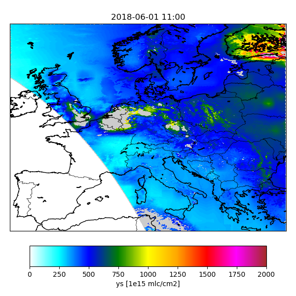
By default the catalogue creator simply creates a map with the value of the a variable on the track. Optionally settings could be used to specifiy a different unit, or the value range for the colorbar:

! convert units:
cso.tutorial.catalogue.var.yr.units          :  1e15 mlc/cm2
! style:
cso.tutorial.catalogue.var.yr.vmin           :   0.0
cso.tutorial.catalogue.var.yr.vmax           :  10.0

Figures are saved to files with the basename of the original orbit file and the plotted variable:

/Scratch/CSO/catalogue/2018/06/01/S5p_RPRO_NO2_20180601_0300_yr.png
                                  S5p_RPRO_NO2_20180601_0300_ys.png
                                  :

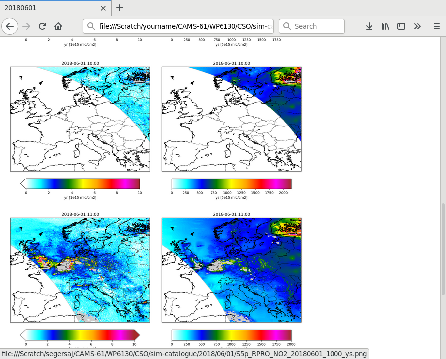
To search for interesting features in the data, the Indexer class could be used to create index pages. Configuration could look like:

! index creation task:
cso.s5p.no2.sim-catalogue.task.index.class     :  utopya.Indexer
cso.s5p.no2.sim-catalogue.task.index.args      :  '${PWD}/rc/cso-s5p.rc', \
                                                    rcbase='cso.s5p.no2.sim-catalogue-index'

When succesful, the index creator displays an url that could be loaded in a browser:

Browse to:
  file:///Scratch/CSO/sim-catalogue/index.html

Gradient computation

In variational assimilations it is necessary to have a gradient forcing field. The gradient forcing field has the shape of a concentration field, and is added to a gradient field at the time to which observations are assigned. The field is filled using entities from the observation operator:

\[\bar{\mathbf{g}} ~=~ \mathbf{H}^T\ \mathbf{R}^{-1}\ \left(\ \mathbf{y}_s\ -\ \mathbf{y}\ \right)\]

The forward observation operator \(\mathbf{H}\) applies after each other a horizontal mapping, a vertical mapping, and an averaging kernel application; the transposed (or adjoint) operator \(\mathbf{H}^T\) should then apply in reveresed order the adjoint operators: adjoint kernel application, adjoint vertical mapping, and adjoint horizontal mapping:

\[\mathbf{H}^T ~=~ \mathbf{G}^T\ \mathbf{V}^T\ \mathbf{A}^T\]

Configuration of adjoint operations

The adjoint operations are applied after each other on entities defined per pixel (profiles). The intermediate entities could be computed using Formula application. For this, the following variables from the satellite product should be available:

! data variables:
!   hp   : half-level pressures for retrieval layers
!   yr   : retrieval
!   vr   : retrieval error variances
!   A    : averaging kernel
tutorial.S5p.no2.dvars             :  hp yr vr A

At run time, the following state variables should be created:

! state varaiables to be created:
!   mod_conc   : model concentrations       over footprint
!   mod_hp     : model half-level pressures over footprint
!   xs         : simulated profile at apriori layers
!   ys         : simulated retrieval profile
!   eps        : gradient forcing at retrieval layers
!   f          : gradient forcing at apriori layers
!   mod_g      : gradient forcing at model layers
tutorial.S5p.no2.vars        :  mod_conc mod_hp xs ys eps f mod_g

The variables mod_conc, mod_hp, xs, and ys are all created from a forward simulation of the retrieval product, as defined in the previous sections. The variables eps, f, and mod_g are the (intermediate) variables for the gradient computation.

The gradient forcing at retreival layers could be computed using the ‘R^{-1} ( ys - y )’ formula:

\[\mathbf{\epsilon} ~=~ \mathbf{R}^{-1}\ \left(\ \mathbf{y}_s\ -\ \mathbf{y}\ \right)\]

The formula ‘A^T eps’ is then used to apply the adjoint kernel:

\[\mathbf{f} ~=~ \mathbf{A}^{T}\ \mathbf{\epsilon}\]

The adjoint vertical mapping is implemented in the ‘LayerAverageAdj( mod_hp, hp, f )’ formula:

\[\mathbf{g} ~=~ \mathbf{V}^T\ \mathbf{f}\]

The equation for the adjoint of the horizontal mapping is then:

\[\bar{\mathbf{g}} ~=~ \mathbf{G}^T\ \mathbf{g}\]

This ioperator should be implemented using the horizontal mapping indices and weights that were used for the observation simuationl as described in the Horizontal mapping section. The adjoint of the mapping disributes fractions of the per-pixel forcingss \(g_p\) over the grid cells that it covers:

\[\bar{g}(i_k,j_k) ~=~ \sum\limits_{\forall\ p\ :\ (i_k,j_k)\in K_p} g_p\ w_{p,k}/w_p\]

The code could look like:

! gradient array:
real                    ::  grad(nlon,nlat,nz)
! pixel array:
real, pointer           ::  mod_g(:,:)        ! (:,npix)

! loop variables:
integer                 ::  ipix
integer                 ::  iw

! from observation simulation:
!   integer     ::  npix         ! number of pixels
!   integer     ::  areas(npix)  ! pixel area
!   integer     ::  nw(npix)     ! number of mapping weights
!   integer     ::  iw0(npix)    ! offset in mapping arrays
!   integer     ::  ii(:)        ! (nmapping)  grid cell index
!   integer     ::  jj(:)        ! (nmapping)  grid cell index
!   integer     ::  ww(:)        ! (nmapping)  overlapping area

! get pointer to gradient array with shape (nz,npix):
call sstate%GetData( status, name='mod_g', data1=mod_g )
if (status/=0) stop

! init gradient:
grad = 0.0

! any pixel?
if ( npix > 0 ) then

  ! loop over pixels:
  do ipix = 1, npix
    ! any source contributions?
    if ( nw(ipix) > 0 ) then
      ! loop over source contributions:
      do iw = iw0(ipix)+1, iw0(ipix)+nw(ipix)
        ! add contribution:
        grad(ii(iw),jj(iw),:) = grad(ii(iw),jj(iw),:) + mod_g(:,ipix) * ww(iw)/areas(ipix)
      end do ! iw
    end if ! nw > 0
  end do ! ipix

end if ! npix > 0

Tutorial with adjoint test

A tutorial program tutorial_oper_adj-test.F90 is available to illustrate the adjoint observation operator. Make the executable using (see also Compiling and running tutorial):

cd src
make tutorial_oper_adj-test.x
cd ..

The settings used by this executable are in:

tutorial_oper_adj-test.F90

The tutorial progam will perform adjoint tests to check that the adjoint operation is indeed the transpose of the forward operation. The thest is performed using the following steps:

• First two model states are created, preferably filled with random numbers:

  \[\bar{\mathbf{c}}_1,~\bar{\mathbf{c}}_2\]

• Then two forward observation simulations are created:

  \[\begin{split}\mathbf{y}_{s1} &= \mathbf{y}_{a0}\ +\ \mathbf{H}\ \bar{\mathbf{c}}_1 \\ \mathbf{y}_{s2} &= \mathbf{y}_{a0}\ +\ \mathbf{H}\ \bar{\mathbf{c}}_2\end{split}\]

  The observation simulations are computed from the states using the obseration operator \(\mathbf{H}\), which denotes the linear part of the mapping from the state; in addition, an offset \(\mathbf{y}_{a0}\) might be included too, typically due to presence of an a priori profile in the retrieval product.

• A random forcing \(\mathbf{\epsilon}\) is created, to which the adjoint observation operator is applied; the resuult is a gradient model state:

  \[\bar{\mathbf{g}} ~=~ \mathbf{H}^T\ \mathbf{\epsilon}\]

• The adjoint test then checks whether the implemented \(\mathbf{H}^T\) operation is indeed the transpose of the implemented \(\mathbf{H}\) operation. If this is true, the following dot products should be equal:

  \[\begin{split}\mathbf{\epsilon}^T\ \left(\ \mathbf{y}_{s2}\ -\ \mathbf{y}_{s1}\ \right) &= \mathbf{\epsilon}^T\ \left(\ \mathbf{H}\ \bar{\mathbf{c}}_2\ -\ \mathbf{H}\ \bar{\mathbf{c}}_1\ \right) \\ &= \mathbf{\epsilon}^T\ \mathbf{H}\ \left(\ \bar{\mathbf{c}}_2\ -\ \bar{\mathbf{c}}_1\ \right) \\ &= \left(\ \mathbf{H}^T\ \mathbf{\epsilon}\ \right)^T\ \left(\ \bar{\mathbf{c}}_2\ -\ \bar{\mathbf{c}}_1\ \right) \\ &= \bar{\mathbf{g}}^T\ \left(\ \bar{\mathbf{c}}_2\ -\ \bar{\mathbf{c}}_1\ \right)\end{split}\]

  The two dot products are compared in absolute and relative sense; the difference should be in the order of machine precission. Running the test with double precission is advised if this is not the standard already.

  In case the test fails (dot products are substantially different), then it is useful to know which part of the adjoint operator is not implemented correctly. The adjoint test is therefore not only applied over the entire operation, but also to the underlying operators:

  • for horizontal mapping:

    \[\begin{split}\mathbf{c}_1 &= \mathbf{G}\ \bar{\mathbf{c}}_{1} \\ \mathbf{c}_2 &= \mathbf{G}\ \bar{\mathbf{c}}_{2}\end{split}\]

    with adjoint operation:

    \[\bar{\mathbf{g}} ~=~ \mathbf{G}^T \mathbf{g}\]

    compare:

    \[\mathbf{g}^T\ \left(\ \mathbf{c}_{2}\ -\ \mathbf{c}_{1}\ \right) ~=~ \bar{\mathbf{g}}^T\ \left(\ \bar{\mathbf{c}}_2\ -\ \bar{\mathbf{c}}_1\ \right)\]

  • for vertical mapping:

    \[\begin{split}\mathbf{x}_{s1} &= \mathbf{V}\ \mathbf{c}_{1} \\ \mathbf{x}_{s2} &= \mathbf{V}\ \mathbf{c}_{2}\end{split}\]

    with adjoint operation:

    \[\mathbf{g}^T ~=~ \mathbf{V}^T\ \mathbf{f}\]

    compare:

    \[\mathbf{f}^T\ \left(\ \mathbf{x}_{s2}\ -\ \mathbf{x}_{s1}\ \right) ~=~ \mathbf{g}^T\ \left(\ \mathbf{c}_{2}\ -\ \mathbf{c}_{1}\ \right)\]

  • for kernel application:

    \[\begin{split}\mathbf{y}_{s1} &= \mathbf{A}\ \mathbf{x}_{s1} \\ \mathbf{y}_{s2} &= \mathbf{A}\ \mathbf{x}_{s2}\end{split}\]

    with adjoint operation:

    \[\mathbf{f} ~=~ \mathbf{A}^T \mathbf{\epsilon}\]

    compare:

    \[\mathbf{\epsilon}^T\ \left(\ \mathbf{y}_{s2}\ -\ \mathbf{y}_{s1}\ \right) ~=~ \mathbf{f}^T\ \left(\ \mathbf{x}_{s2}\ -\ \mathbf{x}_{s1}\ \right)\]

  If the test fails for one of these operations, the problem should be searched in there. But keep in mind that also the test itself might not be implemented correctly (yet), for example in a domain-decomposition …