Sentinel-5p NO2 data processing
This chapter describes the tasks performed for processing Sentinel-5p NO2 data.
Product description
The product guides can be found at:
Sentinel-5p / Products and Algoritms
L2__NO2___,PUM-NO2Product User Manual
Features:
The retrieval product is a column density (mol/m2), which will be treated by CSO as a profile with \(n_r=1\) layers:
\[\mathbf{y}_r\]The simulation of a retrieval product from a model state does not require an apriori profile, and should be computed from:
\[\mathbf{y}_s ~=~ \mathbf{A}^{trop}\ \mathbf{V}\mathbf{G}\ \mathbf{x}\]where:
\(\mathbf{y}_s\) is the simulated retrieval (mol/m2) defined on \(n_r=1\) layers;
\(\mathbf{A}^{trop}\) is the tropospheric averaging kernel matrix with shape \((n_r,n_a)\), with \(n_a\) the number of a priori layers;
\(\mathbf{x}\) is the atmospheric state, which probably consists of a 3D array of NO2 concentrations;
operators \(\mathbf{G}\) and \(\mathbf{V}\) together compute a simulated profile at the \(n_a\) a priori layers from the state, using horizontal (\(\mathbf{G}\)) and vertical (\(\mathbf{V}\)) mappings; units should be the same as the retrieval product (mol/m2).
In case \(\mathbf{x}^{true}\) is the true atmoshperic state, the retrieval error is quantified by the retrieval error covariance \(\mathbf{R}\) (in this scalar product a variance):
\[\mathbf{y}_s ~-~ \mathbf{A}^{trop}\ \mathbf{V}\mathbf{G}\ \mathbf{x}^{true} ~\sim~ \mathcal{N}\left(\mathbf{o},\mathbf{R}^{trop}\right)\]The retrieval status and quality is indicated by the
qa_value. The recommended minimum is 0.75, this excludes cloudy scenes and other problematic retrievals.Multiple cloud fraction variables are present. For filtering NO2 retrievals, the best variable seems:
float cloud_fraction_crb_nitrogendioxide_window(time, scanline, ground_pixel) ;
  proposed_standard_name = "effective_cloud_area_fraction_assuming_fixed_cloud_albedo" ;
  units                  = "1" ;
  long_name              = "Cloud fraction at 440 nm for NO2 retrieval" ;
  radiation_wavelength   = 440.f ;
  assumed_cloud_albedo   = 0.8f ;
Averaging kernels
The tropospheric averaging kernel should be computed from:
using the following variables from the data file:
- \(\mathbf{A}(n_r,n_a)\) is the total column averaging kernel [1];
note that in the current product \(n_r=1\)
\(M\) is the scalar total column airmass factor [1];
\(M^{trop}(n_r)\) is the tropspheric column airmass factor [1]; in this product it is a sclar;
\(l_{tp}\) is the index of the layer holding the tropopause in the a priori profile [number within \(1,..,n_a\)].
The air mass factor is the ratio between the optical thickness of the NO2 in the slant column (observed part of the irradiated atmosphere) and the optical thickness in the vertical column (perpendicular to the earth’s surface). The air mass factors in the product are based on simulations with the TM5 global atmospheric model, which are currently on a rather coarse resolution of 0.5x0.5 degrees horizontally. As a consquence, the air mass factors do not represent the strong gradients that are present near emission hot spots. Luckily, as long as the averaging kernels are used to simulate a retrieved product, a comparison between the simulation and the retrieval is independend of the air mass factors that are used.
This property can be exploited to replace the original retrieval and tropospheric averaging kernel (that depend on the TM5 a priori profile) by alternative versions that are based on other simulations, for example a high-resolution CTM. Concentration maps of the retrieval or its simulation will then likely to show more detail where strong gradients are present. Following the formulas in the Product User Manual, the first step is to compute an alternative tropospheric airmass factor using the alternative a priori profile \(\hat{\mathbf{x}}_a\) (note that this equation is only valid for \(n_r=1\)):
This is used to obtain the alternative retrieval and tropospheric averaging kernel as scalled versions of the original variables:
A simulation of the retrieval from the same model concentrations becomes:
Thus, if the concentration profile of a local model is used as a priori instead of the TM5 profile, then the simulated tropospheric column retrieval is actually the full tropospheric model column.
The impact of the local airmass factor is illustrated in the figure below. The top row shows an example of the original retrieval product and simulation by the LOTOS-EUROS model using standard tropospheric kernel. The bottom row shows the same using local airmass factor corrections, which shows sharper gradients.
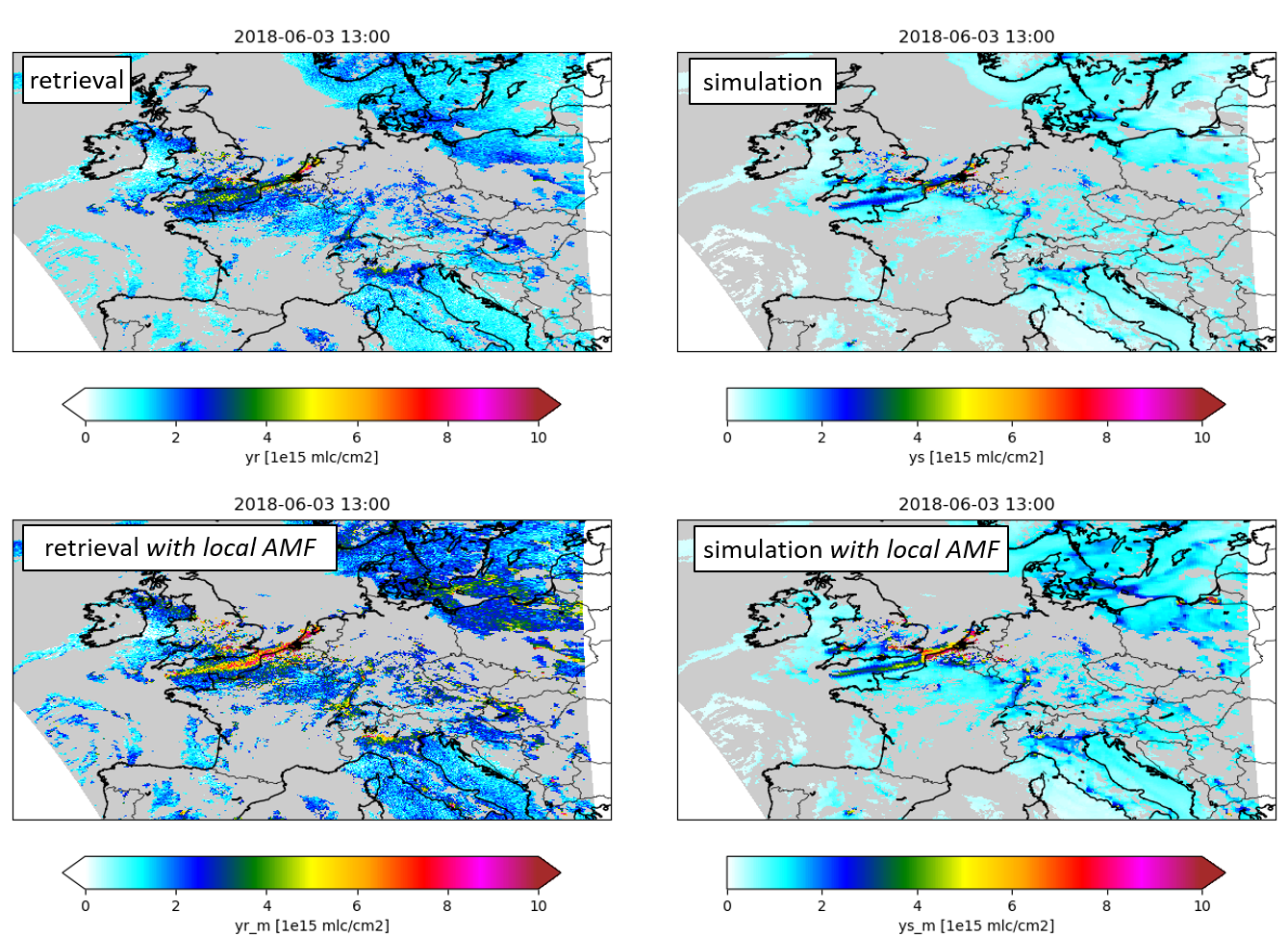
Illustration of airmass factor correction. Top row: original NO2 retrieval and LOTOS-EUROS simulation using standard tropospheric kernel. Bottom row: similar using airmass factor correction.
Note that an assimilation procedure is indifferent of the scaling, since the same factor is applied to observations, the simulations, and the representation error. Using the notation:
for the combined horizontal, vertical, and kernell operators, the result of the analysis update that is used in the Kalman filter is:
and the observation part of the cost function used in variational assimilation is:
Both equations remain the same when using the local-airmass correction, assuming that the retrieval error covariance is used for the observation-representation-error \(R\). If \(R\) is constructed using other contributions, for example based on grid cell representation, then these contributions should be revised following the new (airmass corrected) observations and simulations.
Inquire Sentinel-5p/NO2 archives
S5p/NO2 observations from KNMI are available from at least these sources:
Copernicus Open Access Hub; see the cso_scihub module module for a detailed description.
Product Algorithm Laboratory; see the cso_pal module module for a detailed description.
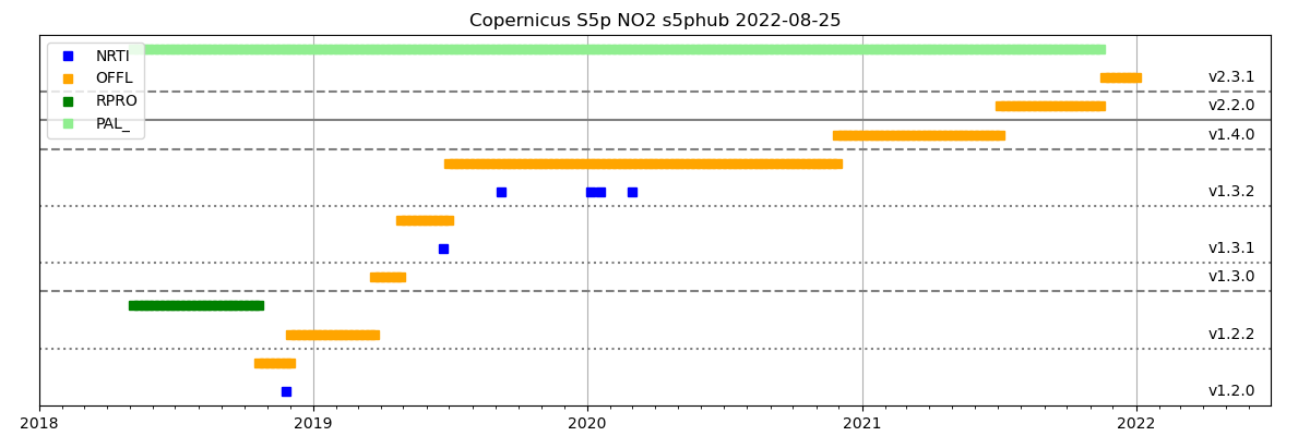
Data is available for different processing streams, each identified by a 4-character key:
NRTI: Near real time, available with a day after observation;OFFL: Offline, available within weeks after observations;RPRO: re-processing of all previously made observations;PAL_: re-processed data stored on the Product Algorithm Laboratory portal.
The portals provide data files created with the same retrieval algorithm, but most recent data (latest processor version) might be available on only one of the portals. It is therefore necessary to first inquire both archives to see which data is available where, and what the version numbers are.
The CSO_SciHub_Inquire class is available to inquire the
Copernicus Open Access Hub. The settings used by this class allow selection
on for example time range and intersection area.
The result is a csv file which with columns for keywords such orbit number and processor version,
as well as the filename of the data and the url that should be used to actually download the data:
orbit;start_time;end_time;processing;collection;processor_version;filename;href
21497;2021-12-06 14:05:54;2021-12-06 15:47:24;OFFL;02;020301;S5P_OFFL_L2__NO2____20211206T140554_20211206T154724_21497_02_020301_20211208T043331.nc;https://s5phub.copernicus.eu/dhus/odata/v1/Products('d9d33ffa-9fe5-43cc-b5a1-b65c22e874ad')/$value
21852;2021-12-31 14:37:39;2021-12-31 16:19:09;OFFL;02;020301;S5P_OFFL_L2__NO2____20211231T143739_20211231T161909_21852_02_020301_20220102T064010.nc;https://s5phub.copernicus.eu/dhus/odata/v1/Products('ff5c922c-450c-43db-97e4-f46bdd55ffb2')/$value
:
See the section on File name convention in the Product User Manual for the meaning of all parts of the filename.
A similar class CSO_PAL_Inquire class is available to list the content
of the Product Algorithm Laboratory portal. Also this will produce a table file.
To visualize what is available from the various portals, the
CSO_Inquire_Plot could be used to create an overview figure:
The jobtree configuration to inquire the portals and create the overview figure could look like:
! single step:
cso.s5p.no2.inquire-scihub.class              :  utopya.UtopyaJobStep
! inquire from portals, plot overview:
cso.s5p.no2.inquire.tasks                     :  scihub pal plot
!~ create table with available files on portal:
cso.s5p.no2.inquire.scihub.class              :  cso.CSO_SciHub_Inquire
cso.s5p.no2.inquire.scihub.args               :  '${PWD}/config/EMEP/cso-s5p-no2.rc', \
                                                      rcbase='cso.s5p.no2.inquire-s5phub'
!~ create table with available files on portal:
cso.s5p.no2.inquire.pal.class                 :  cso.CSO_PAL_Inquire
cso.s5p.no2.inquire.pal.args                  :  '${PWD}/config/EMEP/cso-s5p-no2.rc', \
                                                      rcbase='cso.s5p.no2.inquire-pal'
!~ create plot of available versions:
cso.s5p.no2.inquire.plot.class                :  cso.CSO_Inquire_Plot
cso.s5p.no2.inquire.plot.args                 :  '${PWD}/config/EMEP/cso-s5p-no2.rc', \
                                                      rcbase='cso.s5p.no2.inquire-plot'
Conversion to CSO format
The ‘cso.s5p.no2.convert’ task converts orbit files downloaded from a portal into a CSO format.
Files are downloaded from a portal if not present locally yet; eventually they are also removed after conversion to avoid that the portal is completely mirrored.
To save storage, only selected pixels are included in the converted files,
for example only those within some region or cloud free pixels.
The selection criteria are defined in the settings, and added
to the ‘history’ attribute of the created files as reminder.
The work is done by the CSO_S5p_Convert class,
which is initialized using the settings file:
! task initialization:
cso.s5p.no2.convert.class     :  cso.CSO_S5p_Convert
cso.s5p.no2.convert.args      :  '${PWD}/config/ESA-S5p/cso-s5p-no2.rc', rcbase='cso.s5p.no2.convert'
See the class documentation for the general configuration, below some specific choices are described. The example is based on the S5p NO2 file from which the header is available in:
Pixel selection
The CSO_S5p_Convert class calls the S5p_File.SelectPixels() method
to create a pixel selection mask for the input file.
The selection is done using one or more filters.
First provide a list of filter names:
cso.s5p.no2.convert.filters : lons lats valid quality cloud_fraction
Then provide for each filter the the input variable to be used for testing,
as a path name in the input file.
The next settings is the type of filter to be used, see the S5p_File.SelectPixels() for supported types,
and the other settings required by the type.
The following is an example of a selection on longitude:
cso.s5p.no2.convert.filter.lons.var                :  Geolocation Fields/Longitude
cso.s5p.no2.convert.filter.lons.type               :  minmax
cso.s5p.no2.convert.filter.lons.minmax             :  -30.0 45.0
cso.s5p.no2.convert.filter.lons.units              :  degrees_east
Variable specification
The target file is created as an CSO_S5p_File object.
It’s AddSelection method is called with the input object as argument,
and this will copy the selected pixels for variables specified in the settings.
The variable specification starts with a list with variable names to be created in the target file:
cso.s5p.no2.convert.output.vars   :  longitude longitude_bounds \
                                    latitude latitude_bounds \
                                     track_longitude track_longitude_bounds \
                                     track_latitude  track_latitude_bounds \
                                     time \
                                     vcd vcd_errvar \
                                     pressure kernel_trop amf amf_trop l_tp nla \
                                     qa_value \
                                     cloud_fraction
For each variable settings should be specified that describe the shape of the variable
and how it should be filled from the input.
See the AddSelection description for all options,
here we show some examples.
The longitude and latitude variables are copied almost directly out of the source files,
the only change that is applied is the selection of pixels.
All original attributes are copied, except for the bound attribite since that would
give warnings from the CF-compliance checker:
cso.s5p.no2.convert.output.var.longitude.dims                   :   pixel
cso.s5p.no2.convert.output.var.longitude.from                   :   PRODUCT/longitude
cso.s5p.no2.convert.output.var.longitude.attrs                  :   { 'bounds' : None }

cso.s5p.no2.convert.output.var.latitude.dims                    :   pixel
cso.s5p.no2.convert.output.var.latitude.from                    :   PRODUCT/latitude
cso.s5p.no2.convert.output.var.latitude.attrs                   :   { 'bounds' : None }
Also the locations of the pixels in the original track are copied, since these are useful when creating plots. These cannot be copied directly but require special processing:
cso.s5p.no2.convert.output.var.track_longitude.dims             :   track_scan track_pixel
cso.s5p.no2.convert.output.var.track_longitude.special          :   track_longitude
cso.s5p.no2.convert.output.var.track_longitude.from             :   PRODUCT/longitude
cso.s5p.no2.convert.output.var.track_longitude.attrs            :   { 'bounds' : None }

cso.s5p.no2.convert.output.var.track_latitude.dims              :   track_scan track_pixel
cso.s5p.no2.convert.output.var.track_latitude.special           :   track_latitude
cso.s5p.no2.convert.output.var.track_latitude.from              :   PRODUCT/latitude
cso.s5p.no2.convert.output.var.track_latitude.attrs             :   { 'bounds' : None }
The observattion times are constructed from time steps relative to a reference time; this requires special processing too:
cso.s5p.no2.convert.output.var.time.dims                        :   pixel
cso.s5p.no2.convert.output.var.time.special                     :   time-delta
cso.s5p.no2.convert.output.var.time.tref                        :   PRODUCT/time
cso.s5p.no2.convert.output.var.time.dt                          :   PRODUCT/delta_time
The observed vertical column density could be copied directly.
The target shape is (pixel,retr) where retr is the number of layers in the retrieval product (1 in this case):
! vertical column density:
cso.s5p.no2.convert.output.var.vcd.dims                         :   pixel retr
cso.s5p.no2.convert.output.var.vcd.from                         :   PRODUCT/nitrogendioxide_tropospheric_column
In the converted files, the retrieval error is always expressed as a (co)variance matrix, to facilitate (future) conversion of profile products. In this example, it is filled from the square of the error standard deviation:
! error variance in vertical column density (after application of kernel),
! fill with single element 'covariance matrix', from square of standard error:
! use dims with different names to avoid that cf-checker complains:
cso.s5p.no2.convert.output.var.vcd_errvar.dims                  :   pixel retr retr0
cso.s5p.no2.convert.output.var.vcd_errvar.special               :   square
cso.s5p.no2.convert.output.var.vcd_errvar.from                  :   PRODUCT/nitrogendioxide_tropospheric_column_precision_kernel
!~ skip standard name, modifier "standard_error" is not valid anymore:
cso.s5p.no2.convert.output.var.vcd_errvar.attrs                 :   { 'standard_name' : None }
The averaging kernel is applied on atmospheric layers, defined by pressure levels. In this product the pressure levels are defined using hybride-sigma-pressure coordinates, and this requires special processing:
! Convert from hybride coefficient bounds in (2,nlev) aray to 3D half level pressure:
cso.s5p.no2.convert.output.var.pressure.dims                    :   pixel layeri
cso.s5p.no2.convert.output.var.pressure.special                 :   hybounds_to_pressure
cso.s5p.no2.convert.output.var.pressure.sp                      :   PRODUCT/SUPPORT_DATA/INPUT_DATA/surface_pressure
cso.s5p.no2.convert.output.var.pressure.hyab                    :   PRODUCT/tm5_constant_a
cso.s5p.no2.convert.output.var.pressure.hybb                    :   PRODUCT/tm5_constant_b
cso.s5p.no2.convert.output.var.pressure.units                   :   Pa
Averaging kernels are converted to matrices with shape (layer,retr).
Here, the averaging kernels of the tropospheric product should be computed using a ratio
between total and tropospheric airmass factors:
! description:
!   kernel := averaging_kernel * amf/amft
cso.s5p.no2.convert.output.var.kernel_trop.dims                 :   pixel layer retr
cso.s5p.no2.convert.output.var.kernel_trop.special              :   kernel_trop
cso.s5p.no2.convert.output.var.kernel_trop.avk                  :   PRODUCT/averaging_kernel
cso.s5p.no2.convert.output.var.kernel_trop.amf                  :   PRODUCT/air_mass_factor_total
cso.s5p.no2.convert.output.var.kernel_trop.amft                 :   PRODUCT/air_mass_factor_troposphere
cso.s5p.no2.convert.output.var.kernel_trop.troplayer            :   PRODUCT/tm5_tropopause_layer_index
cso.s5p.no2.convert.output.var.kernel_trop.attrs                :   { 'coordinates' : None, 'ancillary_variables' : None }
For the airmass factor correction, the airmass factors and the tropopause level are needed:
! (total) airmass factor:
cso.s5p.no2.convert.output.var.amf.dims                         :   pixel retr
cso.s5p.no2.convert.output.var.amf.from                         :   PRODUCT/air_mass_factor_total
cso.s5p.no2.convert.output.var.amf.attrs                        :   { 'coordinates' : None, 'ancillary_variables' : None }

! tropospheric airmass factor:
cso.s5p.no2.convert.output.var.amf_trop.dims                    :   pixel retr
cso.s5p.no2.convert.output.var.amf_trop.from                    :   PRODUCT/air_mass_factor_troposphere
cso.s5p.no2.convert.output.var.amf_trop.attrs                   :   { 'coordinates' : None, 'ancillary_variables' : None }

! number of apriori layers in retrieval layer,
! enforce that it is stored as a short integer:
cso.s5p.no2.convert.output.var.nla.dims                         :   pixel retr
cso.s5p.no2.convert.output.var.nla.dtype                        :   i2
cso.s5p.no2.convert.output.var.nla.from                         :   PRODUCT/tm5_tropopause_layer_index
cso.s5p.no2.convert.output.var.nla.attrs                        :   { 'coordinates' : None, 'ancillary_variables' : None }
Other variables can be copied directly:
! quality flag:
cso.s5p.no2.convert.output.var.qa_value.dims                   :   pixel
cso.s5p.no2.convert.output.var.qa_value.from                   :   PRODUCT/qa_value
!~ skip some attributes, cf-checker complains ...
cso.s5p.no2.convert.output.var.qa_value.attrs                  :   { 'valid_min' : None, 'valid_max' : None }

! cloud property:
cso.s5p.no2.convert.output.var.cloud_fraction.dims             :   pixel
cso.s5p.no2.convert.output.var.cloud_fraction.from             :   PRODUCT/SUPPORT_DATA/INPUT_DATA/cloud_fraction_crb
cso.s5p.no2.convert.output.var.cloud_fraction.attrs            :   { 'coordinates' : None, 'source' : None }

! cloud property:
cso.s5p.no2.convert.output.var.cloud_radiance_fraction.dims    :   pixel
cso.s5p.no2.convert.output.var.cloud_radiance_fraction.from    :   PRODUCT/SUPPORT_DATA/DETAILED_RESULTS/cloud_radiance_fraction_nitrogendioxide_window
cso.s5p.no2.convert.output.var.cloud_radiance_fraction.attrs   :   { 'coordinates' : None, 'ancillary_variables' : None }
Output files
The name of the target files should be specified with a directory and filename; the later could include a template for the orbit number:
! output directory and filename:
! - times are taken from mid of selection, rounded to hours
! - use '%{orbit}' for orbit number
cso.s5p.no2.convert.output.dir          :  /Scratch/CSO/S5p/RPRO/NO2/Europe/%Y/%m
cso.s5p.no2.convert.output.filename     :  S5p_RPRO_NO2_%{orbit}.nc
A flag is read to decide if existing files should be renewed or kept:
cso.s5p.no2.convert.renew : True
The target file is created as an CSO_S5p_File object.
It’s AddSelection method is called with the input object as argument,
and this will copy the selected pixels for variables specified in the settings.
The Write method creates the file.
Global attributes for the target file should be specified with:
! global attributes:
cso.s5p.no2.convert.output.attrs               :  format Conventions author institution email
!
cso.s5p.no2.convert.output.attr.format         :  1.0
cso.s5p.no2.convert.output.attr.Conventions    :  CF-1.7
cso.s5p.no2.convert.output.attr.author         :  Your Name
cso.s5p.no2.convert.output.attr.institution    :  CSO
cso.s5p.no2.convert.output.attr.email          :  Your.Name@cso.org
Listing file
A listing file contains the names of the converted orbit files, and the time range of pixels in the file:
filename                     ;start_time                   ;end_time                     ;orbit
2018/06/S5p_RPRO_NO2_03272.nc;2018-06-01T01:32:46.673000000;2018-06-01T01:36:12.948000000;03272
2018/06/S5p_RPRO_NO2_03273.nc;2018-06-01T03:12:53.649000000;2018-06-01T03:17:43.082000000;03273
2018/06/S5p_RPRO_NO2_03274.nc;2018-06-01T04:52:43.586000000;2018-06-01T04:59:12.377000000;03274
:
This file will be used by the observation operator to selects orbits with pixels valid for a desired time range.
In the settings, define the name of the file to be created:
! csv file that will hold records per file with:
! - timerange of pixels in file
! - orbit number
<rcbase>.file        :   /Scratch/CSO/S5p/listing-NO2-Europe.csv
An existing listing files is not replaced, unless the following flag is set:
! renew table?
<rcbase>.renew           :  True
Orbit files are searched within a timerange:
<rcbase>.timerange.start        :  2018-06-01 00:00
<rcbase>.timerange.end          :  2018-06-03 23:59
Specify filename filters to search for orbit files; the patterns are relative to the basedir of the listing file, and might contain templates for the time values. Multiple patterns could be defined; if for a certain orbit number more than one file is found, the first match is used. This could be explored to create a listing that combines reprocessed data with near-real-time data:
<rcbase>.patterns            :  RPRO/NO2/Europe/%Y/%m/S5p_*.nc \
                                OFFL/NO2/Europe/%Y/%m/S5p_*.nc
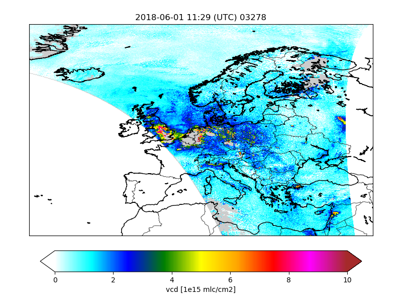
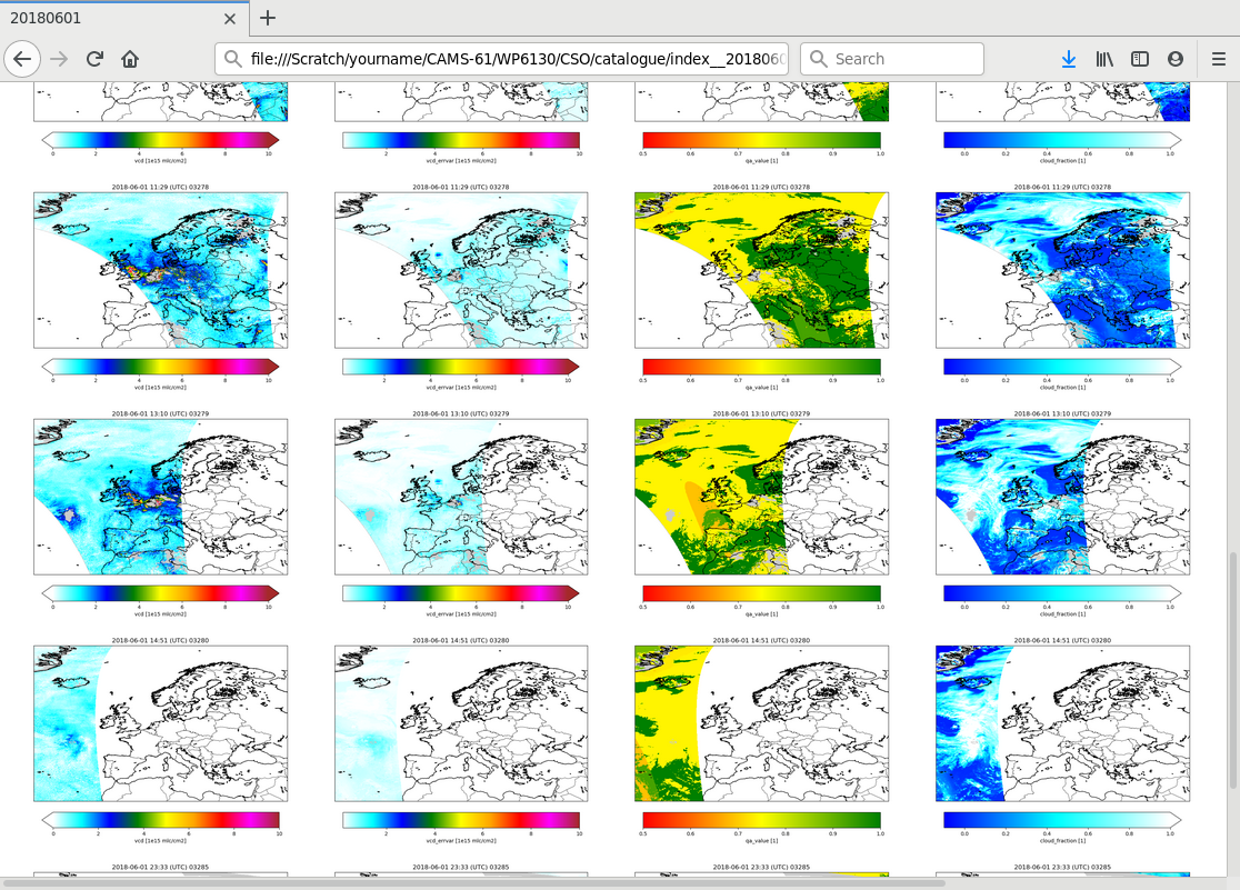
Catalogue
The CSO_Catalogue class could be used
to create a catalogue of images for the converted files.
Configuration could look like:
! catalogue creation task:
cso.s5p.no2.catalogue.task.figs.class  :  cso.CSO_Catalogue
cso.s5p.no2.catalogue.task.figs.args   :  '${PWD}/config/ESA-S5p/cso-s5p-no2.rc', \
                                            rcbase='cso.s5p.no2.catalogue'
The configuration describes where to find a listing file with orbits,
which variables should be plot, the colorbar properties, etc.
See CSO_Catalogue class description for how
the settings in general look like.
The class creates figures for a list of variables:
! variables to be plotted:
cso.s5p.no2.catalogue.vars                    :  vcd vcd_errvar qa_value \
                                                    cloud_fraction cloud_radiance_fraction
By default the catalogue creator simply creates a map with the value of the a variable on the track. Optionally settings could be used to specifiy a different unit, or the value range for the colorbar:
! convert units:
cso.s5p.no2.catalogue.var.vcd.units          :  1e15 mlc/cm2
! style:
cso.s5p.no2.catalogue.var.vcd.vmin           :   0.0
cso.s5p.no2.catalogue.var.vcd.vmax           :  10.0
Figures are saved to files with the basename of the original orbit file and the plotted variable:
/Scratch/CSO/catalogue/2018/06/01/S5p_RPRO_NO2_03278__vcd.png
                                  S5p_RPRO_NO2_03278__qa_value.png
                                  :
To search for interesting features in the data,
the Indexer class could be used to create index pages.
Configuration could look like:
! index creation task:
cso.s5p.no2.catalogue.task.index.class     :  utopya.Indexer
cso.s5p.no2.catalogue.task.index.args      :  '${PWD}/config/ESA-S5p/cso-s5p-no2.rc', \
                                               rcbase='cso.s5p.no2.catalogue-index'
When succesful, the index creator displays an url that could be loaded in a browser:
Browse to:
  file:///Scratch/CSO/catalogue/index.html
Configuration of observation operator
The observation operator described in chapter ‘Observation operator’ requires settings from an rcfile.
First specify the (relative) location of the listing file with orbit file names and time ranges:
! template for listing with converted files:
<rcbase>.listing           : ../S5p/RPRO/NO2/CAMS/listing.csv
The S5p data contains data defined on orbit tracks, this should be read from the files:
! also read info on original track (T|F)?
! if enabled, this will be stored in the output too:
<rcbase>.with_track        :  T
The operator should read variables from the data files that are needed to simulate a retrieval from the model arrays. This includes for example the pressures that define the a priori layers, the averaging kernel, and for this product, the airmass factor and tropopause level. Specify a list of names for these variables:
! data variables:
tutorial.S5p.no2.dvars             :  hp yr vr A M nla
Example settings:
! half-level pressures:
!~ dimensions, copied from data file:
tutorial.S5p.no2.dvar.hp.dims      :  layeri
!~ source variable:
tutorial.S5p.no2.dvar.hp.source    :  pressure

! retrieval:
!~ dimensions, copied from data file:
tutorial.S5p.no2.dvar.yr.dims      :  retr
!~ source variable:
tutorial.S5p.no2.dvar.yr.source    :  vcd

! retrieval error covariance:
!~ dimensions, copied from data file:
tutorial.S5p.no2.dvar.vr.dims      :  retr retr
!~ source variable:
tutorial.S5p.no2.dvar.vr.source    :  vcd_errvar

! kernel:
!~ dimensions, copied from data file:
tutorial.S5p.no2.dvar.A.dims       :  retr layer
!~ source variable:
tutorial.S5p.no2.dvar.A.source     :  kernel_trop

! tropospheric airmass factor
!~ dimensions, copied from data file:
tutorial.S5p.no2.dvar.M.dims       :  retr
!~ source variable:
tutorial.S5p.no2.dvar.M.source     :  amf_trop

! number of apriori layers in retrieval layer:
!~ dimensions, copied from data file:
tutorial.S5p.no2.dvar.nla.dims     :  retr
!~ source variable:
tutorial.S5p.no2.dvar.nla.source   :  nla
For the simulated values, also define a list of variable names that should be created:
! state varaiables to be put out from model:
tutorial.S5p.no2.vars                         :  mod_conc mod_hp mod_tcc mod_cc hx ys shx M_m A_m yr_m ys_m
Example settings:
! model concentration profile:
!~ model layer dimension:
tutorial.S5p.no2.var.mod_conc.dims            :  model_layer
!~ standard attributes:
tutorial.S5p.no2.var.mod_conc.attrs           :  long_name units
tutorial.S5p.no2.var.mod_conc.attr.long_name  :  model NO2 concentrations
tutorial.S5p.no2.var.mod_conc.attr.units      :  ppb

! model hpentration profile:
!~ model layer interfaces:
tutorial.S5p.no2.var.mod_hp.dims              :  model_layeri
!~ standard attributes:
tutorial.S5p.no2.var.mod_hp.attrs             :  long_name units
tutorial.S5p.no2.var.mod_hp.attr.long_name    :  model pressure at layer interfaces
tutorial.S5p.no2.var.mod_hp.attr.units        :  Pa

! total cloud cover:
!~ no extra dimensions:
tutorial.S5p.no2.var.mod_tcc.dims             :
!~ standard attributes:
tutorial.S5p.no2.var.mod_tcc.attrs            :  long_name units
tutorial.S5p.no2.var.mod_tcc.attr.long_name   :  total cloud cover
tutorial.S5p.no2.var.mod_tcc.attr.units       :  1

! cloud cover profiles:
!~ model layer dimension:
tutorial.S5p.no2.var.mod_cc.dims              :  model_layer
!~ standard attributes:
tutorial.S5p.no2.var.mod_cc.attrs             :  long_name units
tutorial.S5p.no2.var.mod_cc.attr.long_name    :  cloud cover
tutorial.S5p.no2.var.mod_cc.attr.units        :  1

! model concentrations at apriori layers:
!~ apriori layers:
tutorial.S5p.no2.var.xs.dims                  :  layer
!~ how computed:
tutorial.S5p.no2.var.xs.formula               :  LayerAverage( hp, mod_hp, mod_conc )
tutorial.S5p.no2.var.xs.formula_terms         :  hp: hp mod_hp: mod_hp mod_conc: mod_conc
!~ standard attributes:
tutorial.S5p.no2.var.xs.attrs                 :  long_name units
tutorial.S5p.no2.var.xs.attr.long_name        :  model simulations at apriori layers
tutorial.S5p.no2.var.xs.attr.units            :  mol m-2

! simulated retrievals
!~ retrieval layers:
tutorial.S5p.no2.var.ys.dims                  :  retr
!~ how computed:
tutorial.S5p.no2.var.ys.formula               :  A x
tutorial.S5p.no2.var.ys.formula_terms         :  A: A x: hx
!~ standard attributes:
tutorial.S5p.no2.var.ys.attrs                 :  long_name units
tutorial.S5p.no2.var.ys.attr.long_name        :  simulated retrieval
tutorial.S5p.no2.var.ys.attr.units            :  mol m-2

! partial columns as sum over apriori layers
!~ retrieval layers:
tutorial.S5p.no2.var.Sx.dims                 :  retr
!~ how computed:
tutorial.S5p.no2.var.Sx.formula              :  PartialColumns( nla, x )
tutorial.S5p.no2.var.Sx.formula_terms        :  nla: nla x: hx
!~ standard attributes:
tutorial.S5p.no2.var.Sx.attrs                :  long_name units
tutorial.S5p.no2.var.Sx.attr.long_name       :  tropospheric column in local model
tutorial.S5p.no2.var.Sx.attr.units           :  mol m-2

! airmass factor from local model
!~ retrieval layers:
tutorial.S5p.no2.var.M_m.dims                 :  retr
!~ how computed:
tutorial.S5p.no2.var.M_m.formula              :  AltAirMassFactor( M, A, x, Sx )
tutorial.S5p.no2.var.M_m.formula_terms        :  M: M A: A x: hx Sx: shx
!~ standard attributes:
tutorial.S5p.no2.var.M_m.attrs                :  long_name units
tutorial.S5p.no2.var.M_m.attr.long_name       :  airmass factors from local model
tutorial.S5p.no2.var.M_m.attr.units           :  1

! kernel using airmass factor from local model
!~ retrieval layers times apriori layers
tutorial.S5p.no2.var.A_m.dims                 :  retr layer
!~ how computed:
tutorial.S5p.no2.var.A_m.formula              :  AltKernel( A, M, M_m )
tutorial.S5p.no2.var.A_m.formula_terms        :  A: A M: M M_m: M_m
!~ standard attributes:
tutorial.S5p.no2.var.A_m.attrs                :  long_name units
tutorial.S5p.no2.var.A_m.attr.long_name       :  averaging kernel using local airmass factors
tutorial.S5p.no2.var.A_m.attr.units           :  1

! retrieval using airmass factor from local model
!~ retrieval layers:
tutorial.S5p.no2.var.yr_m.dims                :  retr
!~ how computed:
tutorial.S5p.no2.var.yr_m.formula             :  AltRetrieval( y, M, M_m )
tutorial.S5p.no2.var.yr_m.formula_terms       :  y: yr M: M M_m: M_m
!~ standard attributes:
tutorial.S5p.no2.var.yr_m.attrs               :  long_name units
tutorial.S5p.no2.var.yr_m.attr.long_name      :  retrieval using local airmass factors
tutorial.S5p.no2.var.yr_m.attr.units          :  mol m-2

! simulated retrievals using airmass factor from local model
!~ retrieval layers:
tutorial.S5p.no2.var.ys_m.dims                 :  retr
!~ how computed:
tutorial.S5p.no2.var.ys_m.formula              :  A x
tutorial.S5p.no2.var.ys_m.formula_terms        :  A: A_m x: hx
!~ standard attributes:
tutorial.S5p.no2.var.ys_m.attrs                :  long_name units
tutorial.S5p.no2.var.ys_m.attr.long_name       :  simulated retrieval based on local airmass factors
tutorial.S5p.no2.var.ys_m.attr.units           :  mol m-2
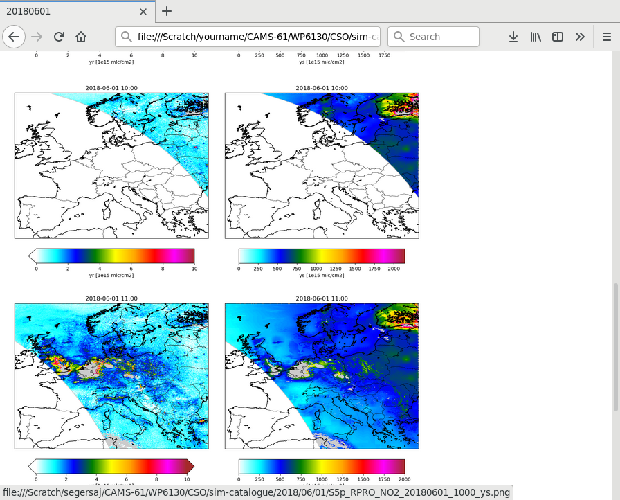
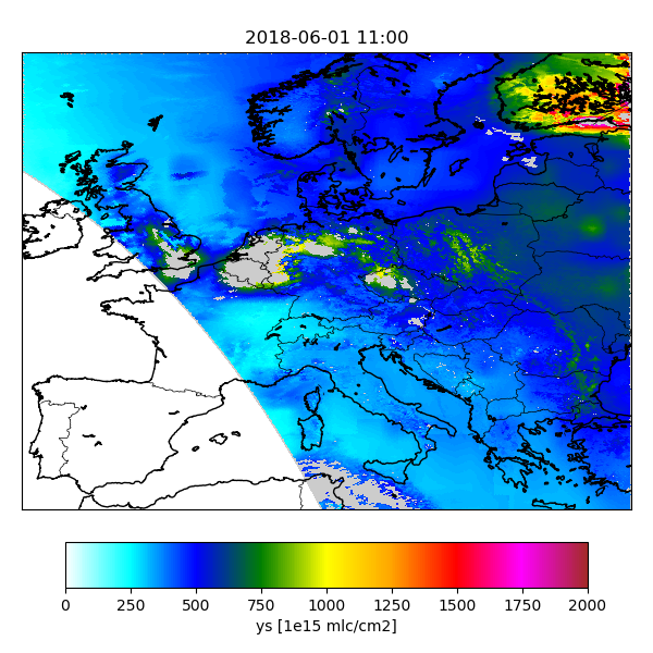
Sim-Catalogue
The CSO_SimCatalogue class could be used
to create a catalogue of images for the converted files.
Configuration could look like:
! catalogue creation task:
cso.s5p.no2.sim-catalogue.task.class          :  cso.CSO_SimCatalogue
cso.s5p.no2.sim-catalogue.task.args           :  '${PWD}/config/ESA-S5p/cso-s5p-TRACER.rc', \
                                                  rcbase='cso.s5p.no2.sim-catalogue'
The configuration describes where to find a listing file with orbits,
which variables should be plot, the colorbar properties, etc.
See CSO_SimCatalogue class description for how
the settings in general look like.
The class creates figures for a list of variables:
! variables to be plotted:
cso.s5p.no2.catalogue.vars                    :  yr ys
By default the catalogue creator simply creates a map with the value of the a variable on the track. Optionally settings could be used to specifiy a different unit, or the value range for the colorbar:
! variable:
cso.s5p.no2.sim-catalogue.var.yr.source          :  data:vcd
! convert units:
cso.s5p.no2.sim-catalogue.var.yr.units           :  1e15 mlc/cm2
! style:
cso.s5p.no2.sim-catalogue.var.yr.vmin            :   0.0
cso.s5p.no2.sim-catalogue.var.yr.vmax            :  50.0

! variable:
cso.s5p.no2.sim-catalogue.var.ys.source          :  state:y
! convert units:
cso.s5p.no2.sim-catalogue.var.ys.units           :  1e15 mlc/cm2
! style:
cso.s5p.no2.sim-catalogue.var.ys.vmin            :   0.0
cso.s5p.no2.sim-catalogue.var.ys.vmax            :  50.0
Figures are saved to files with the basename of the original orbit file and the plotted variable:
file://Scratch/cso-catalogue/NO2//2018/06/01/S5p_RPRO_NO2_20180601_1200_yr.png
                                             S5p_RPRO_NO2_20180601_1200_ys.png
To search for interesting features in the data,
the Indexer class could be used to create index pages.
Configuration could look like:
! index creation task:
cso.s5p.no2.catalogue.task.index.class     :  utopya.Indexer
cso.s5p.no2.catalogue.task.index.args      :  '${PWD}/config/ESA-S5p/cso-s5p-no2.rc', \
                                               rcbase='cso.s5p.no2.catalogue-index'
When succesful, the index creator displays an url that could be loaded in a browser:
Browse to:
  file://Scratch/cso-catalogue/NO2/index.html