Sentinel-5p NO2 super-observations processing
This chapter describes the tasks performed for processing Sentinel-5p NO2 data that have been averaged to a regular grid.
Settings for the processing are in:
Product description
See S5p-NO2 Product Description for the original product.
The TROPOMI NO2 Super-Obsersvations have been provided by KNMI (Henk Eskes) for use in the CAMS_81 project, work package on soil-NOx emissions. The product consists of NO2 retrievals and auxilary data (kernels) averaged over a regular 0.5x0.5 grid.
Each file contains a gridded version of a single orbit:
TROPOMI/NO2/superobs/201805_0.5deg/compressed/s5p_no2_rpro_v1.2.2_superobs_ll_0.5deg_02833.nc
The attributes of the file describe how the data was created:
originating S5p/NO2 product:
product_version      = "v 1.2.2, reprocessing March 2019, RPRO" ;
S5P_NO2_file_name    = "S5P_RPRO_L2__NO2____20180501T014123_20180501T032451_02833_01_010202_20190201T165715.nc" ;
S5P_NO2_orbit_number = 2833 ;
selection filters for pixels:
filter_min_QA_value = 0.75f ;
filter_max_QA_value = 1.1f ;
settings for creation of super observations:
superobs_setting_modelStratVcdError = 0.15f ; superobs_setting_minimal_coverage = 0.5f ; superobs_setting_correlation_factor = 0.15f ; superobs_setting_meanVariabilityFactor = 0.5f ;
Features:
The retrieval product is a column density (mol/m2), which will be treated by CSO as a profile with \(n_r=1\) layers:
\[\mathbf{y}_r\]The simulation of a retrieval product from a model state does not require an apriori profile, and should be computed from:
\[\mathbf{y}_s ~=~ \mathbf{A}^{trop}\ \mathbf{V}\mathbf{G}\ \mathbf{x}\]where:
\(\mathbf{y}_s\) is the simulated retrieval (mol/m2) defined on \(n_r=1\) layers;
\(\mathbf{A}^{trop}\) is the tropospheric averaging kernel matrix with shape \((n_r,n_a)\), with \(n_a\) the number of a priori layers;
\(\mathbf{x}\) is the atmospheric state, which probably consists of a 3D array of NO2 concentrations;
operators \(\mathbf{G}\) and \(\mathbf{V}\) together compute a simulated profile at the \(n_a\) a priori layers from the state, using horizontal (\(\mathbf{G}\)) and vertical (\(\mathbf{V}\)) mappings; units should be the same as the retrieval product (mol/m2).
In case \(\mathbf{x}^{true}\) is the true atmoshperic state, the retrieval error is quantified by the retrieval error covariance \(\mathbf{R}\) (in this scalar product a variance):
\[\mathbf{y}_s ~-~ \mathbf{A}^{trop}\ \mathbf{V}\mathbf{G}\ \mathbf{x}^{true} ~\sim~ \mathcal{N}\left(\mathbf{o},\mathbf{R}^{trop}\right)\]
The files contain 3 different variables with error descriptions:
float no2_superobs_uncertainty(lat, lon) ;
        long_name = "NO2 tropospheric column superobservation uncertainty, TROPOMI sensor, including representation error" ;
        units     = "1e-6 mol m^-2" ;

float no2_superobs_uncertainty_representation(lat, lon) ;
        long_name = "NO2 tropospheric column superobservation uncertainty, TROPOMI sensor, only representation error" ;
        units     = "1e-6 mol m^-2" ;

float average_uncertainty(lat, lon) ;
        long_name = "NO2 tropospheric column superobservation uncertainty, TROPOMI sensor, average over individual observation" ;
        units     = "1e-6 mol m^-2" ;
Averaging kernels
The tropospheric averaging kernel is already present in the files, and does not need to be computed as described in Averaging kernels.
As described overthere too, a scaling could be applied using the tropospheric air mass factor (which is supplied in the data too), for better comparison between retrievals and simulations.
Conversion to CSO format
The ‘cso.s5p_no2_superobs.convert’ task creates netCDF files with selected pixels,
for example only those within some region or cloud free pixels.
The selection criteria are defined in the settings, and added
to the ‘history’ attribute of the created files as reminder.
The work is done by the CSO_S5p_SuperObs_Convert class,
which is initialized using the settings file:
! convert:
cso.s5p_no2_superobs.convert.task.class     :  cso.CSO_S5p_SuperObs_Convert
cso.s5p_no2_superobs.convert.task.args      :  '%{rcfile}', rcbase='cso.s5p_no2_superobs.convert'
See the class documentation for the general configuration, below some specific choices are described.
Input files
The files are searched in subdirectories including templates for time fields; also specify filename patterns to be matched:
! input directory:
cso.s5p_no2_superobs.convert.files.dir         :  /Scratch/TROPOMI/NO2/superobs/%Y%m_0.5deg/compressed

! filename filters (space seperated list):
cso.s5p_no2_superobs.convert.files.filters     :  s5p_no2_rpro_v1.2.2_superobs_ll_0.5deg_*.nc
Example content of input file:
Pixel selection
The CSO_S5p_SuperObs_Convert class calls the S5p_SuperObs_File.SelectPixels() method
to create a pixel selection mask for the input file.
The selection is done using one or more filters.
The original pixels have already been filtered on quality flag.
Here it is therefore sufficient to select on valid data, which will select only the grid cells
that have been covered by an orbit:
cso.s5p_no2_superobs.convert.filters : valid
Then provide for each filter the the input variable to be used for testing,
as a path name in the input file.
The next settings is the type of filter to be used, see the S5p_SuperObs_File.SelectPixels() for supported types,
and the other settings required by the type.
The following is shows the selection on valid data:
! skip pixel with "no data", use the retrieved variable to check:
cso.s5p_no2_superobs.convert.filter.valid.var       :  no2_superobs
cso.s5p_no2_superobs.convert.filter.valid.type      :  valid
Variable specification
The target file is created as an CSO_S5p_SuperObs_File object.
It’s AddSelection method is called with the input object as argument,
and this will copy the selected pixels for variables specified in the settings.
The variable specification starts with a list with variable names to be created in the target file:
cso.s5p_no2_superobs.convert.output.vars  :  longitude longitude_bounds \
                                             latitude  latitude_bounds \
                                             track_longitude track_longitude_bounds \
                                             track_latitude  track_latitude_bounds \
                                             vcd vcd_errvar \
                                             pressure kernel_trop amf_trop nla
For each variable settings should be specified that describe the shape of the variable
and how it should be filled from the input.
See the AddSelection description for all options,
here we show some examples.
The longitude and latitude variables should contain the pixel centers.
Pixels are in this case grid cells of 0.5x0.5 degrees that actually have data.
The lon and lat arrays in the file are 1D axes for the entire grid,
and these should be selected for the pixel variables:
! center longitudes, sampled from 1D axes:
cso.s5p_no2_superobs.convert.output.var.longitude.dims                   :   pixel
cso.s5p_no2_superobs.convert.output.var.longitude.from                   :   lon

! center latitudes, sampled from 1D axes:
cso.s5p_no2_superobs.convert.output.var.latitude.dims                    :   pixel
cso.s5p_no2_superobs.convert.output.var.latitude.from                    :   lat
Corner values per pixel are for example used for plotting. Here these are created using interpolation/extrapolation of the center locations:
! corner longitudes, compute from centers:
cso.s5p_no2_superobs.convert.output.var.longitude_bounds.dims            :   pixel corner
cso.s5p_no2_superobs.convert.output.var.longitude_bounds.special         :   longitude_to_bounds
cso.s5p_no2_superobs.convert.output.var.longitude_bounds.from            :   lon
cso.s5p_no2_superobs.convert.output.var.longitude_bounds.units           :   degrees_east

! corner latitudes, compute from centers:
cso.s5p_no2_superobs.convert.output.var.latitude_bounds.dims             :   pixel corner
cso.s5p_no2_superobs.convert.output.var.latitude_bounds.special          :   latitude_to_bounds
cso.s5p_no2_superobs.convert.output.var.latitude_bounds.from             :   lat
cso.s5p_no2_superobs.convert.output.var.latitude_bounds.units            :   degrees_north
In addition, also an obrbit track is defined, since this is used for map plots. For the gridded averages, the track is simply the regular lon/lat grid. The values are derived from the lon/lat coordinates:
! track is entire grid, copy longitudes:
cso.s5p_no2_superobs.convert.output.var.track_longitude.dims             :   track_scan track_pixel
cso.s5p_no2_superobs.convert.output.var.track_longitude.from             :   lon
cso.s5p_no2_superobs.convert.output.var.track_longitude.units            :   degrees_east

! track is entire grid, copy longitudes:
cso.s5p_no2_superobs.convert.output.var.track_latitude.dims              :   track_scan track_pixel
cso.s5p_no2_superobs.convert.output.var.track_latitude.from              :   lat
cso.s5p_no2_superobs.convert.output.var.track_latitude.units             :   degrees_north

! corner longitudes, compute from centers:
cso.s5p_no2_superobs.convert.output.var.track_longitude_bounds.dims      :   track_scan track_pixel corner
cso.s5p_no2_superobs.convert.output.var.track_longitude_bounds.special   :   longitude_to_bounds
cso.s5p_no2_superobs.convert.output.var.track_longitude_bounds.from      :   lon
cso.s5p_no2_superobs.convert.output.var.track_longitude_bounds.units     :   degrees_east

! corner latitudes, compute from centers:
cso.s5p_no2_superobs.convert.output.var.track_latitude_bounds.dims       :   track_scan track_pixel corner
cso.s5p_no2_superobs.convert.output.var.track_latitude_bounds.special    :   latitude_to_bounds
cso.s5p_no2_superobs.convert.output.var.track_latitude_bounds.from       :   lat
cso.s5p_no2_superobs.convert.output.var.track_latitude_bounds.units      :   degrees_north
The observed vertical column density could be copied directly.
The target shape is (pixel,retr) where retr is the number of layers in the retrieval product (1 in this case):
! vertical column density:
cso.s5p_no2_superobs.convert.output.var.vcd.dims                         :   pixel retr
cso.s5p_no2_superobs.convert.output.var.vcd.from                         :   no2_superobs
In the converted files, the retrieval error is always expressed as a (co)variance matrix, to facilitate (future) conversion of profile products. In this example, it is filled from the square of the error standard deviation:
! error variance in vertical column density (after application of kernel),
! fill with single element 'covariance matrix', from square of standard error:
! use dims with different names to avoid that cf-checker complains:
cso.s5p_no2_superobs.convert.output.var.vcd_errvar.dims                  :   pixel retr retr0
cso.s5p_no2_superobs.convert.output.var.vcd_errvar.special               :   square
cso.s5p_no2_superobs.convert.output.var.vcd_errvar.from                  :   no2_superobs_uncertainty
The averaging kernel is applied on atmospheric layers, defined by pressure levels. In this product the pressure levels are defined using hybride-sigma-pressure coordinates, and this requires special processing:
! Convert from hybride coefficient bounds in (2,nlev) aray to 3D half level pressure:
cso.s5p_no2_superobs.convert.output.var.pressure.dims                    :   pixel layeri
cso.s5p_no2_superobs.convert.output.var.pressure.special                 :   hybounds_to_pressure
cso.s5p_no2_superobs.convert.output.var.pressure.sp                      :   surface_pressure
cso.s5p_no2_superobs.convert.output.var.pressure.hyab                    :   tm5_constant_a
cso.s5p_no2_superobs.convert.output.var.pressure.hybb                    :   tm5_constant_b
cso.s5p_no2_superobs.convert.output.var.pressure.units                   :   Pa
The tropospheric averaging kernels are included:
! tropospheric kernel
cso.s5p_no2_superobs.convert.output.var.kernel_trop.dims                 :   pixel layer retr
cso.s5p_no2_superobs.convert.output.var.kernel_trop.from                 :   kernel_troposphere
For the airmass factor correction, the airmass factors and the tropopause level are needed; the later is derived by checking the non-zero values in the kernel profiles:
! tropospheric airmass factor:
cso.s5p_no2_superobs.convert.output.var.amf_trop.dims                    :   pixel retr
cso.s5p_no2_superobs.convert.output.var.amf_trop.from                    :   amf_trop_superobs

! number of apriori layers in retrieval layer, count using kernel profile:
cso.s5p_no2_superobs.convert.output.var.nla.dims                        :   pixel retr
cso.s5p_no2_superobs.convert.output.var.nla.special                     :   kernel_trop_to_nla
cso.s5p_no2_superobs.convert.output.var.nla.kernel_trop                 :   kernel_troposphere
Output files
The name of the target files should be specified with a directory and filename; the later could include a template for the orbit number:
! output directory and filename:
! - times are taken from mid of selection, rounded to hours
! - use '%{orbit}' for orbit number
cso.s5p_no2_superobs.convert.output.dir                     :  /Scratch/CSO-data/S5p/NO2/superobs/%Y/%m
cso.s5p_no2_superobs.convert.output.filename                :  S5p_NO2_superobs_%{orbit}.nc
A flag is read to decide if existing files should be renewed or kept:
cso.s5p_no2_superobs.convert.renew : True
The target file is created as an CSO_S5p_SuperObs_File object.
It’s AddSelection method is called with the input object as argument,
and this will copy the selected pixels for variables specified in the settings.
The Write method creates the file.
Global attributes for the target file should be specified with:
! global attributes:
cso.s5p_no2_superobs.convert.output.attrs               :  format Conventions author institution email
!
cso.s5p_no2_superobs.convert.output.attr.format         :  1.0
cso.s5p_no2_superobs.convert.output.attr.Conventions    :  CF-1.7
cso.s5p_no2_superobs.convert.output.attr.author         :  Your Name
cso.s5p_no2_superobs.convert.output.attr.institution    :  CSO
cso.s5p_no2_superobs.convert.output.attr.email          :  Your.Name@cso.org
In addition, the global attribtues from the original file are copied too, preceeded by a specified prefix:
! copy global attributes? specify filename filters:
cso.s5p_no2_superobs.convert.output.gattrs.filters      :  *
! prefix for new attributes:
cso.s5p_no2_superobs.convert.output.gattrs.prefix       :  source__
Listing file
A listing file contains the names of the converted orbit files, and the time range of pixels in the file:
filename                                      ;start_time         ;end_time           ;orbit
NO2/superobs/2018/05/S5p_NO2_superobs_02833.nc;2018-05-01 02:03:58;2018-05-01 02:56:14;02833
NO2/superobs/2018/05/S5p_NO2_superobs_02834.nc;2018-05-01 03:45:28;2018-05-01 04:43:52;02834
NO2/superobs/2018/05/S5p_NO2_superobs_02835.nc;2018-05-01 05:26:57;2018-05-01 06:25:21;02835
:
This file will be used by the observation operator to selects orbits with pixels valid for a desired time range.
In the settings, define the name of the file to be created:
! csv file that will hold records per file with:
! - timerange of pixels in file
! - orbit number
<rcbase>.file        :   /Scratch/CSO-data/S5p/listing-NO2-superobs.csv
An existing listing files is not replaced, unless the following flag is set:
! renew table?
<rcbase>.renew           :  True
Orbit files are searched within a timerange:
<rcbase>.timerange.start        :  2018-05-01 00:00
<rcbase>.timerange.end          :  2018-12-31 23:59
Specify filename filters to search for orbit files; the patterns are relative to the basedir of the listing file, and might contain templates for the time values. Multiple patterns could be defined; if for a certain orbit number more than one file is found, the first match is used. This could be explored to create a listing that combines reprocessed data with near-real-time data:
<rcbase>.patterns : NO2/superobs/%Y/%m/S5p_*.nc
The superobs files do not have a time coordinate, and therefore this is not present in the CSO converted files either. Instead, take the time range from the copied global attributes:
! adhoc: use attributes to extract timerange from?
cso.s5p_no2_superobs.listing.use_attrs           :  True
! if True, define names:
cso.s5p_no2_superobs.listing.attr_tr1            :  source__time_coverage_start
cso.s5p_no2_superobs.listing.attr_tr2            :  source__time_coverage_end
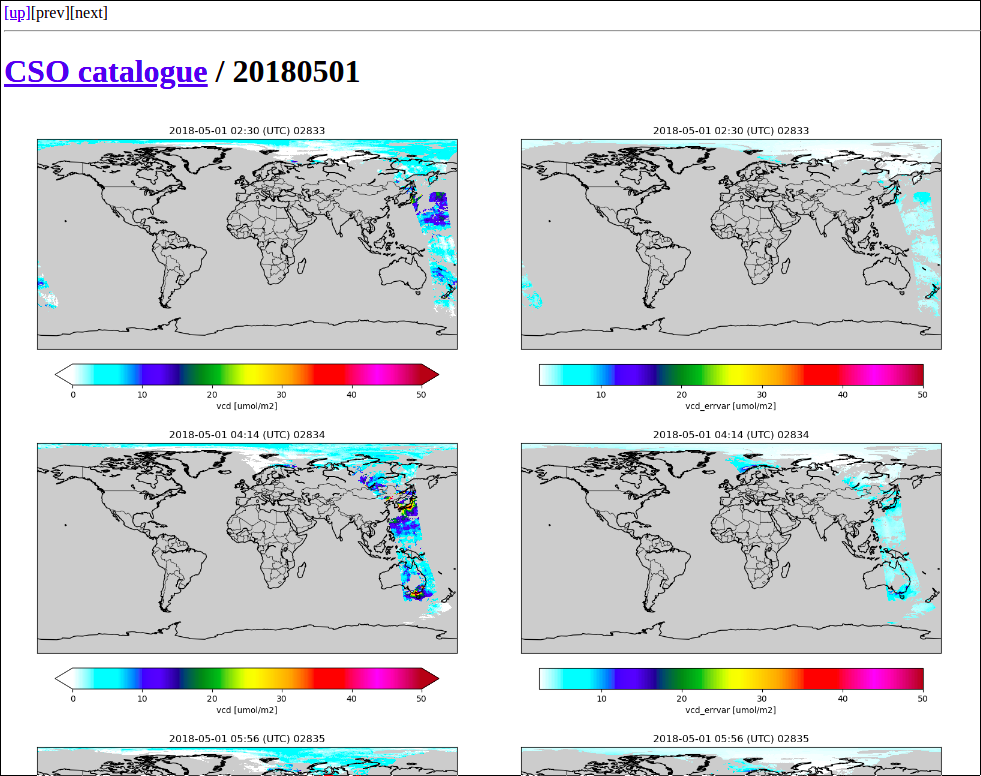
Catalogue
The CSO_Catalogue class could be used
to create a catalogue of images for the converted files.
Configuration could look like:
! catalogue creation task:
cso.s5p_no2_superobs.catalogue.figs.class              :  cso.CSO_Catalogue
cso.s5p_no2_superobs.catalogue.figs.args               :  '%{rcfile}', rcbase='cso.s5p_no2_superobs.catalogue-figs'
The configuration describes where to find a listing file with orbits,
which variables should be plot, the colorbar properties, etc.
See CSO_Catalogue class description for how
the settings in general look like.
The class creates figures for a list of variables:
! variables to be plotted:
cso.s5p_no2_superobs.catalogue.vars                    :  vcd vcd_errvar
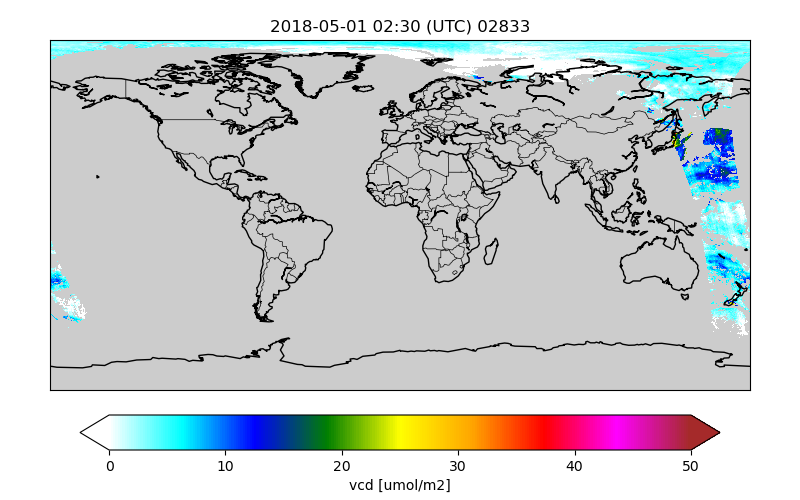
By default the catalogue creator simply creates a map with the value of the a variable on the track. Optionally settings could be used to specifiy a different unit, or the value range for the colorbar:
! convert units:
cso.s5p_no2_superobs.catalogue-figs.var.vcd.units               :  umol/m2
! style:
cso.s5p_no2_superobs.catalogue-figs.var.vcd.vmin                :    0.0
cso.s5p_no2_superobs.catalogue-figs.var.vcd.vmax                :   50.0
Figures are saved to files with the basename of the original orbit file and the plotted variable:
/Scratch/CSO-data-catalogue/2018/05/01/S5p_NO2_superobs_02833__vcd.png
                                       :
To search for interesting features in the data,
the Indexer class could be used to create index pages.
Configuration could look like:
! index creation task:
cso.s5p_no2_superobs.catalogue.index.class             :  utopya.Indexer
cso.s5p_no2_superobs.catalogue.index.args              :  '%{rcfile}', rcbase='cso.s5p_no2_superobs.catalogue-index'
When succesful, the index creator displays an url that could be loaded in a browser:
Browse to:
  file:///Scratch/CSO-data-catalogue/index.html
Configuration of observation operator
The observation operator described in chapter ‘Observation operator’ requires settings from an rcfile.
First specify the (relative) location of the listing file with orbit file names and time ranges:
! template for listing with converted files:
<rcbase>.listing           : /Scratch/CSO-data/S5p/listing-NO2-superobs.csv
The S5p superobs data contains data defined on orbit tracks, which are in this case simply the regular grid; also these should be read from the files:
! also read info on original track (T|F)?
! if enabled, this will be stored in the output too:
<rcbase>.with_track        :  T
The operator should read variables from the data files that are needed to simulate a retrieval from the model arrays. This includes for example the pressures that define the a priori layers, the averaging kernel, and for this product, the airmass factor and tropopause level. Specify a list of names for these variables:
! data variables:
S5p-no2-superobs.dvars             :  hp yr vr A M nla
Example settings:
! half-level pressures:
!~ dimensions, copied from data file:
S5p-no2-superobs.dvar.hp.dims      :  layeri
!~ source variable:
S5p-no2-superobs.dvar.hp.source    :  pressure

! retrieval:
!~ dimensions, copied from data file:
S5p-no2-superobs.dvar.yr.dims      :  retr
!~ source variable:
S5p-no2-superobs.dvar.yr.source    :  vcd

! retrieval error covariance:
!~ dimensions, copied from data file:
S5p-no2-superobs.dvar.vr.dims      :  retr retr
!~ source variable:
S5p-no2-superobs.dvar.vr.source    :  vcd_errvar

! kernel:
!~ dimensions, copied from data file:
S5p-no2-superobs.dvar.A.dims       :  retr layer
!~ source variable:
S5p-no2-superobs.dvar.A.source     :  kernel_trop

! tropospheric airmass factor
!~ dimensions, copied from data file:
S5p-no2-superobs.dvar.M.dims       :  retr
!~ source variable:
S5p-no2-superobs.dvar.M.source     :  amf_trop

! number of apriori layers in retrieval layer:
!~ dimensions, copied from data file:
S5p-no2-superobs.dvar.nla.dims     :  retr
!~ source variable:
S5p-no2-superobs.dvar.nla.source   :  nla
For the simulated values, also define a list of variable names that should be created:
! state varaiables to be put out from model:
S5p-no2-superobs.vars                         :  mod_conc mod_hp xs ys Sx M_m A_m yr_m ys_m
Example settings:
! model concentration profile:
!~ model layer dimension:
S5p-no2-superobs.var.mod_conc.dims            :  model_layer
!~ standard attributes:
S5p-no2-superobs.var.mod_conc.attrs           :  long_name units
S5p-no2-superobs.var.mod_conc.attr.long_name  :  model NO2 concentrations
S5p-no2-superobs.var.mod_conc.attr.units      :  ppb

! model hpentration profile:
!~ model layer interfaces:
S5p-no2-superobs.var.mod_hp.dims              :  model_layeri
!~ standard attributes:
S5p-no2-superobs.var.mod_hp.attrs             :  long_name units
S5p-no2-superobs.var.mod_hp.attr.long_name    :  model pressure at layer interfaces
S5p-no2-superobs.var.mod_hp.attr.units        :  Pa

! model concentrations at apriori layers:
!~ apriori layers:
S5p-no2-superobs.var.xs.dims                  :  layer
!~ how computed:
S5p-no2-superobs.var.xs.formula               :  LayerAverage( hp, mod_hp, mod_conc )
S5p-no2-superobs.var.xs.formula_terms         :  hp: hp mod_hp: mod_hp mod_conc: mod_conc
!~ standard attributes:
S5p-no2-superobs.var.xs.attrs                 :  long_name units
S5p-no2-superobs.var.xs.attr.long_name        :  model simulations at apriori layers
S5p-no2-superobs.var.xs.attr.units            :  mol m-2

! simulated retrievals
!~ retrieval layers:
S5p-no2-superobs.var.ys.dims                  :  retr
!~ how computed:
S5p-no2-superobs.var.ys.formula               :  A x
S5p-no2-superobs.var.ys.formula_terms         :  A: A x: hx
!~ standard attributes:
S5p-no2-superobs.var.ys.attrs                 :  long_name units
S5p-no2-superobs.var.ys.attr.long_name        :  simulated retrieval
S5p-no2-superobs.var.ys.attr.units            :  mol m-2

! partial columns as sum over apriori layers
!~ retrieval layers:
S5p-no2-superobs.var.Sx.dims                  :  retr
!~ how computed:
S5p-no2-superobs.var.Sx.formula               :  PartialColumns( nla, x )
S5p-no2-superobs.var.Sx.formula_terms         :  nla: nla x: hx
!~ standard attributes:
S5p-no2-superobs.var.Sx.attrs                 :  long_name units
S5p-no2-superobs.var.Sx.attr.long_name        :  tropospheric column in local model
S5p-no2-superobs.var.Sx.attr.units            :  mol m-2

! airmass factor from local model
!~ retrieval layers:
S5p-no2-superobs.var.M_m.dims                 :  retr
!~ how computed:
S5p-no2-superobs.var.M_m.formula              :  AltAirMassFactor( M, A, x, Sx )
S5p-no2-superobs.var.M_m.formula_terms        :  M: M A: A x: hx Sx: shx
!~ standard attributes:
S5p-no2-superobs.var.M_m.attrs                :  long_name units
S5p-no2-superobs.var.M_m.attr.long_name       :  airmass factors from local model
S5p-no2-superobs.var.M_m.attr.units           :  1

! kernel using airmass factor from local model
!~ retrieval layers times apriori layers
S5p-no2-superobs.var.A_m.dims                 :  retr layer
!~ how computed:
S5p-no2-superobs.var.A_m.formula              :  AltKernel( A, M, M_m )
S5p-no2-superobs.var.A_m.formula_terms        :  A: A M: M M_m: M_m
!~ standard attributes:
S5p-no2-superobs.var.A_m.attrs                :  long_name units
S5p-no2-superobs.var.A_m.attr.long_name       :  averaging kernel using local airmass factors
S5p-no2-superobs.var.A_m.attr.units           :  1

! retrieval using airmass factor from local model
!~ retrieval layers:
S5p-no2-superobs.var.yr_m.dims                :  retr
!~ how computed:
S5p-no2-superobs.var.yr_m.formula             :  AltRetrieval( y, M, M_m )
S5p-no2-superobs.var.yr_m.formula_terms       :  y: yr M: M M_m: M_m
!~ standard attributes:
S5p-no2-superobs.var.yr_m.attrs               :  long_name units
S5p-no2-superobs.var.yr_m.attr.long_name      :  retrieval using local airmass factors
S5p-no2-superobs.var.yr_m.attr.units          :  mol m-2

! simulated retrievals using airmass factor from local model
!~ retrieval layers:
S5p-no2-superobs.var.ys_m.dims                 :  retr
!~ how computed:
S5p-no2-superobs.var.ys_m.formula              :  A x
S5p-no2-superobs.var.ys_m.formula_terms        :  A: A_m x: hx
!~ standard attributes:
S5p-no2-superobs.var.ys_m.attrs                :  long_name units
S5p-no2-superobs.var.ys_m.attr.long_name       :  simulated retrieval based on local airmass factors
S5p-no2-superobs.var.ys_m.attr.units           :  mol m-2
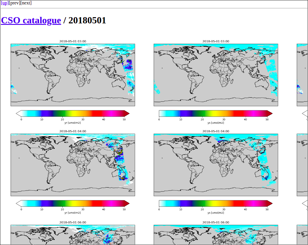
Sim-Catalogue
The CSO_SimCatalogue class could be used
to create a catalogue of images for the converted files.
Configuration could look like:
! catalogue creation task:
cso.s5p_no2_superobs.sim-catalogue.figs.class          :  cso.CSO_SimCatalogue
cso.s5p_no2_superobs.sim-catalogue.figs.args           :  '%{rcfile}', rcbase='cso.s5p_no2_superobs.sim-catalogue-figs'
The configuration describes where to find a listing file with orbits,
which variables should be plot, the colorbar properties, etc.
See CSO_SimCatalogue class description for how
the settings in general look like.
The class creates figures for a list of variables:
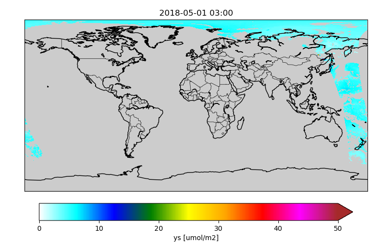
! variables to be plotted:
cso.s5p_no2_superobs.sim-catalogue-figs.vars                :  yr ys yr_m ys_m
By default the catalogue creator simply creates a map with the value of the a variable on the track. Optionally settings could be used to specifiy a different unit, or the value range for the colorbar:
! variable:
cso.s5p_no2_superobs.sim-catalogue-figs.var.yr.source          :  data:yr
! convert units:
cso.s5p_no2_superobs.sim-catalogue-figs.var.yr.units           :  umol/m2
! style:
cso.s5p_no2_superobs.sim-catalogue-figs.var.yr.vmin            :   0.0
cso.s5p_no2_superobs.sim-catalogue-figs.var.yr.vmax            :  50.0

! variable:
cso.s5p_no2_superobs.sim-catalogue-figs.var.ys.source          :  state:ys
! convert units:
cso.s5p_no2_superobs.sim-catalogue-figs.var.ys.units           :  umol/m2
! style:
cso.s5p_no2_superobs.sim-catalogue-figs.var.ys.vmin            :   0.0
cso.s5p_no2_superobs.sim-catalogue-figs.var.ys.vmax            :  50.0
Figures are saved to files with the basename of the original orbit file and the plotted variable:
/Scratch/EMEP-output-catalogue/2018/05/01/EMEP-S5p-NO2_20180501_0300_yr.png
                                          EMEP-S5p-NO2_20180501_0300_ys.png
                                          :
To search for interesting features in the data,
the Indexer class could be used to create index pages.
Configuration could look like:
! index creation task:
cso.s5p_no2_superobs.sim-catalogue.index.class         :  utopya.Indexer
cso.s5p_no2_superobs.sim-catalogue.index.args          :  '%{rcfile}', rcbase='cso.s5p_no2_superobs.sim-catalogue-index'
When succesful, the index creator displays an url that could be loaded in a browser:
Browse to:
  file:///Scratch/EMEP-output-catalogue/NO2/index.html