Sentinel-5p SO2 data processing
This chapter describes the tasks performed for processing Sentinel-5p SO2 data.
Product description
The product guides can be found at:
Sentinel-5p / Products and Algoritms
L2__SO2___,PUM-SO2Product User Manual
Further product details on filters/validation can be found at: https://acp.copernicus.org/articles/20/5591/2020/acp-20-5591-2020.pdf & https://www.nature.com/articles/s41598-019-39279-y
Features:
The retrieval product is a column density (mol/m2), which will be treated by CSO as a profile with \(n_r=1\) layers:
\[\mathbf{y}_r\]The simulation of a retrieval product from a model state does not require an apriori profile, and is denoted with:
\[\mathbf{y}_s ~=~ \mathbf{A}^{trop}\ \mathbf{H}\mathbf{x}\]where:
\(\mathbf{y}_s\) is the simulated retrieval (mol/m2) defined on \(n_r=1\) layers;
\(\mathbf{A}^{trop}\) is the tropospheric averaging kernel matrix with shape \((n_r,n_a)\); in this product, \(n_r=1\) the number of a priori layers; see also the remarks below;
\(\mathbf{x}\) is the atmospheric state, which consists of a 3D array of HCHO concentrations;
\(\mathbf{H}\) extracts a simulated profile from the state using horizontal and vertical interpolation; the result should be defined on the \(n_a\) a priori layers and have the units of the retrieval product (mol/m2).
In case \(\mathbf{x}\) is the true atmoshperic state, the retrieval error is quantified by the retrieval error covariance \(\mathbf{R}\) (in this scalar product a variance):
\[\mathbf{y}_s ~-~ \mathbf{A}^{trop}\ \mathbf{H}\mathbf{x}^{true} ~\sim~ \mathcal{N}\left(\mathbf{o},\mathbf{R}^{trop}\right)\]The retrieval status and quality is indicated by the
qa_value. The recommended minimum is 0.5, this excludes cloudy scenes and other problematic retrievals.
Downloading Sentinel-5p data
Sentinel-5p data could be downloaded from the Copernicus Open Access Hub; see the cso_scihub module module for a detailed description.
The cso_scihub.CSO_SciHub_Download class is available to download data
from this server.
The jobtree configuration could look like:
! download task:
cso.s5p.so2.task.class    :  cso.CSO_SciHub_Download
cso.s5p.so2.task.args     :  '${PWD}/rc/cso-s5p-so2.rc', rcbase='cso.s5p.so2.download-s5phub'
See the class documentation for the general settings that define the download.
Data could be download for different processing streams:
Near real time (NRTI)
Offline (OFFL) : available within weeks after observations;
Reprocessing (RPRO) : re-processing of all previously made observations.
For the Reprocessing stream the download query looks like:
cso.s5p.so2.download-s5phub.query    :   platformname:Sentinel-5     AND \
                                          producttype:L2__SO2___    AND \
                                      processinglevel:L2            AND \
                                       processingmode:Reprocessing
The target directory for downloaded files is specified to have sub-directories per year and month:
! output archive, store in subdirs per month:
cso.s5p.so2.download-s5phub.output.dir   :  ${my.work}/Copernicus/S5P/RPRO/SO2/%Y/%m
The first downloaded files are then:
Copernicus/S5P/RPRO/SO2/2018/06/S5P_RPRO_L2__SO2____20180601T002022_20180601T020350_03272_01_010105_20190207T044248.nc
                                S5P_RPRO_L2__SO2____20180617T034326_20180617T052654_03501_01_010105_20190209T175809.nc
                                S5P_RPRO_L2__SO2____20180601T020152_20180601T034520_03273_01_010105_20190207T052751.nc
                                :
See the section on File name convention in the Product User Manual for the meaning of the fields.
Conversion to CSO format
The ‘cso.s5p.so2.convert’ task creates netCDF files with selected pixels,
for example only those within some region or cloud free pixels.
The selection criteria are defined in the settings, and added
to the ‘history’ attribute of the created files as reminder.
The work is done by the CSO_S5p_Convert class,
which is initialized using the settings file:
! task initialization:
cso.s5p.so2.convert.class     :  cso.CSO_S5p_Convert
cso.s5p.so2.convert.args      :  '${PWD}/rc/cso-s5p-so2.rc', rcbase='cso.s5p.so2.convert'
See the class documentation for the general configuration, below some specific choices are described. The example is based on the S5p SO2 file from which the header is available in:
Pixel selection
The CSO_S5p_Convert class calls the S5p_File.SelectPixels() method
to create a pixel selection mask for the input file.
The selection is done using one or more filters.
First provide a list of filter names:
cso.s5p.so2.convert.filters : lons lats valid quality sza ground_pixel cloud_fraction
Then provide for each filter the the input variable to be used for testing,
as a path name in the input file.
The next settings is the type of filter to be used, see the S5p_File.SelectPixels() for supported types,
and the other settings required by the type.
The following is an example of a selection on longitude:
cso.s5p.so2.convert.filter.lons.var                :  Geolocation Fields/Longitude
cso.s5p.so2.convert.filter.lons.type               :  minmax
cso.s5p.so2.convert.filter.lons.minmax             :  -30.0 45.0
cso.s5p.so2.convert.filter.lons.units              :  degrees_east
Extension to the product guide
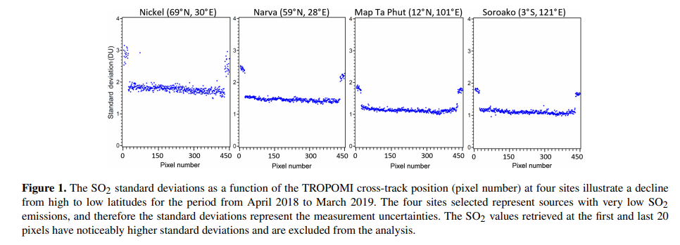
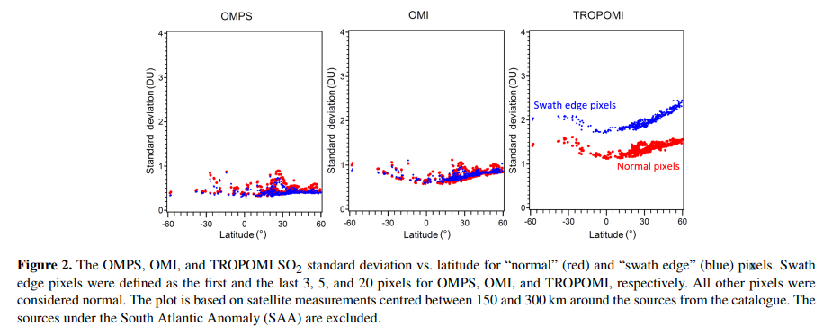
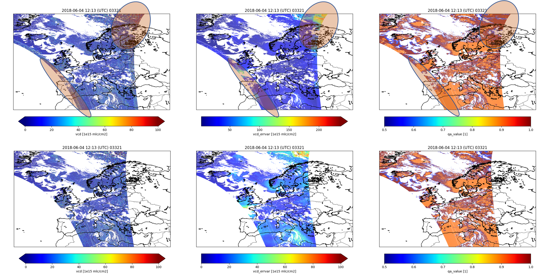
Several publications report extended data criteria beyond the PUMs quality_flags that should be used to ensure data quality. Examples of such are the emission source detection paper by Fioletov et al., 2020 and the volcanic so2 monitoring paper by Theys et al., 2019. Both publications mention the poor quality of observations at the edges of TROPOMI observation swath as well as the reduced quality at high Solar Zenith Angles. The integration time of pixels toward the edge of the swath has been reduced to decrease the pixel size, however this also reduces the overall quality of the observation (SNR). Therefor we advise to only select the pixels with id’s 25-425, and for really strict cases only 50-400. Examples of both the edge pixels and SZA effects are shown in the figures below, with 2 figures from Fioletov et al.,2020 and an example for the SZA based on the CSO results.
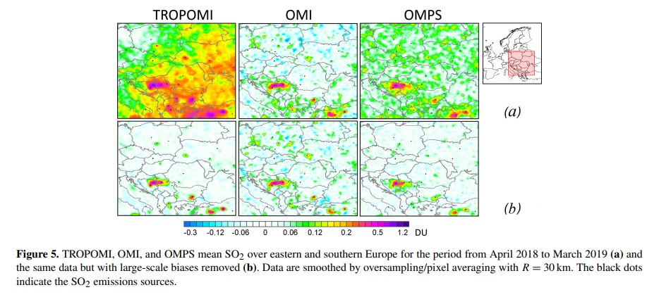
Furthermore, Fioletov et al., 2020 (Fig below) report large-scale biases in the current TROPOMI product, with TROPOMI showing significantly higher total columns, which can be expected to introduce a potential high bias throughout the domain. A solution advised by Fioletov et al is to remove the bias by comparing up- and down-wind values around an SO2 emissions source, but that will not be included in this algorithm.
Variable specification
The target file is created as an CSO_S5p_File object.
It’s AddSelection method is called with the input object as argument,
and this will copy the selected pixels for variables specified in the settings.
The variable specification starts with a list with variable names to be created in the target file:
cso.s5p.so2.convert.output.vars    : longitude longitude_bounds \
                                     latitude latitude_bounds \
                                     track_longitude track_longitude_bounds \
                                     track_latitude  track_latitude_bounds \
                                     time \
                                     pressure kernel qa_value \
                                     vcd vcd_errvar \
                                     detection_flag cloud_fraction solar_zenith_angle ground_pixel
For each variable settings should be specified that describe the shape of the variable
and how it should be filled from the input.
See the AddSelection description for all options,
here we show some examples.
The longitude and latitude variables are copied almost directly out of the source files,
the only change that is applied is the selection of pixels.
All original attributes are copied, except for the bound attribite since that would
give warnings from the CF-compliance checker:
cso.s5p.so2.convert.output.var.longitude.dims                   :   pixel
cso.s5p.so2.convert.output.var.longitude.from                   :   PRODUCT/longitude
cso.s5p.so2.convert.output.var.longitude.attrs                  :   { 'bounds' : None }

cso.s5p.so2.convert.output.var.latitude.dims                    :   pixel
cso.s5p.so2.convert.output.var.latitude.from                    :   PRODUCT/latitude
cso.s5p.so2.convert.output.var.latitude.attrs                   :   { 'bounds' : None }
Also the locations of the pixels in the original track are copied, since these are useful when creating plots. These cannot be copied directly but require special processing:
cso.s5p.so2.convert.output.var.track_longitude.dims             :   track_scan track_pixel
cso.s5p.so2.convert.output.var.track_longitude.special          :   track_longitude
cso.s5p.so2.convert.output.var.track_longitude.from             :   PRODUCT/longitude
cso.s5p.so2.convert.output.var.track_longitude.attrs            :   { 'bounds' : None }

cso.s5p.so2.convert.output.var.track_latitude.dims              :   track_scan track_pixel
cso.s5p.so2.convert.output.var.track_latitude.special           :   track_latitude
cso.s5p.so2.convert.output.var.track_latitude.from              :   PRODUCT/latitude
cso.s5p.so2.convert.output.var.track_latitude.attrs             :   { 'bounds' : None }
The observattion times are constructed from time steps relative to a reference time; this requires special processing too:
cso.s5p.so2.convert.output.var.time.dims                        :   pixel
cso.s5p.so2.convert.output.var.time.special                     :   time-delta
cso.s5p.so2.convert.output.var.time.tref                        :   PRODUCT/time
cso.s5p.so2.convert.output.var.time.dt                          :   PRODUCT/delta_time
The observed vertical column density could be copied directly.
The target shape is (pixel,retr) where retr is the number of layers in the retrieval product (1 in this case):
! vertical column density:
cso.s5p.so2.convert.output.var.vcd.dims                         :   pixel retr
cso.s5p.so2.convert.output.var.vcd.from                         :   PRODUCT/sulfurdioxide_total_vertical_column
In the converted files, the retrieval error is always expressed as a (co)variance matrix, to facilitate (future) conversion of profile products. In this example, it is filled from the square of the error standard deviation:
! error variance in vertical column density (after application of kernel),
! use dims with different names to avoid that cf-checker complains:
cso.s5p.so2.convert.output.var.vcd_errvar.dims                  :   pixel retr
cso.s5p.so2.convert.output.var.vcd_errvar.from                  :   PRODUCT/sulfurdioxide_total_vertical_column_precision
!~ skip standard name, modifier "standard_error" is not valid anymore:
cso.s5p.so2.convert.output.var.vcd_errvar.attrs                 :   { 'standard_name' : None }
The averaging kernel is applied on atmospheric layers, defined by pressure levels. In this product the pressure levels are defined using hybride-sigma-pressure coordinates, and this requires special processing:
! Convert from hybride coefficient bounds in (2,nlev) aray to 3D half level pressure:
cso.s5p.so2.convert.output.var.pressure.dims                    :   pixel layeri
cso.s5p.so2.convert.output.var.pressure.special                 :   hybounds_to_pressure
cso.s5p.so2.convert.output.var.pressure.sp                      :   PRODUCT/SUPPORT_DATA/INPUT_DATA/surface_pressure
cso.s5p.so2.convert.output.var.pressure.hyab                    :   PRODUCT/tm5_constant_a
cso.s5p.so2.convert.output.var.pressure.hybb                    :   PRODUCT/tm5_constant_b
cso.s5p.so2.convert.output.var.pressure.units                   :   Pa
Averaging kernels are converted to matrices with shape (layer,retr).
! description: cso.s5p.so2.convert.output.var.kernel.dims : pixel layer retr cso.s5p.so2.convert.output.var.kernel.from : PRODUCT/SUPPORT_DATA/DETAILED_RESULTS/averaging_kernel
Other variables can be copied directly:
! quality flag:
cso.s5p.so2.convert.output.var.qa_value.dims                   :   pixel
cso.s5p.so2.convert.output.var.qa_value.from                   :   PRODUCT/qa_value
!~ skip some attributes, cf-checker complains ...
cso.s5p.so2.convert.output.var.qa_value.attrs                  :   { 'valid_min' : None, 'valid_max' : None }

! cloud property:
cso.s5p.so2.convert.output.var.cloud_fraction.dims             :   pixel
cso.s5p.so2.convert.output.var.cloud_fraction.from             :   PRODUCT/SUPPORT_DATA/INPUT_DATA/cloud_fraction_crb
cso.s5p.so2.convert.output.var.cloud_fraction.attrs            :   { 'coordinates' : None, 'source' : None }

! detection flag, for observations near known source locations:
cso.s5p.so2.convert.output.var.detection_flag.dims             :   pixel
cso.s5p.so2.convert.output.var.detection_flag.from             :   PRODUCT/SUPPORT_DATA/DETAILED_RESULTS/sulfurdioxide_detection_flag
cso.s5p.so2.convert.output.var.detection_flag.attrs            :   { 'coordinates' : None }
cso.s5p.so2.convert.output.var.detection_flag.dtype            :   i1
Output files
The name of the target files should be specified with a directory and filename; the later could include a template for the orbit number:
! output directory and filename:
! - times are taken from mid of selection, rounded to hours
! - use '%{orbit}' for orbit number
cso.s5p.so2.convert.output.dir          :  /Scratch/CSO/S5p/RPRO/SO2/Europe/%Y/%m
cso.s5p.so2.convert.output.filename     :  S5p_RPRO_SO2_%{orbit}.nc
A flag is read to decide if existing files should be renewed or kept:
cso.s5p.so2.convert.renew : True
The target file is created as an CSO_S5p_File object.
It’s AddSelection method is called with the input object as argument,
and this will copy the selected pixels for variables specified in the settings.
The Write method creates the file.
Global attributes for the target file should be specified with:
! global attributes:
cso.s5p.so2.convert.output.attrs               :  format Conventions author institution email
!
cso.s5p.so2.convert.output.attr.format         :  1.0
cso.s5p.so2.convert.output.attr.Conventions    :  CF-1.7
cso.s5p.so2.convert.output.attr.author         :  Your Name
cso.s5p.so2.convert.output.attr.institution    :  CSO
cso.s5p.so2.convert.output.attr.email          :  Your.Name@cso.org
The conversion also creates (or updates) a listing file with the names of the created files (relative to the listing file), and the time range of pixels in the file:
! csv file that will hold records per file with:
! - timerange of pixels in file
! - orbit number
cso.s5p.hcho.convert.output.listing.file        :  /Scratch/CSO/S5p/listing-SO2-Europe.csv
This file will be used by the observation operator to selects orbits with pixels valid for a desired time range. The listing is a csv file that looks like:
filename                     ;start_time                   ;end_time                     ;orbit
2018/06/S5p_RPRO_SO2_03272.nc;2018-06-01T01:32:46.673000000;2018-06-01T01:36:12.948000000;03272
2018/06/S5p_RPRO_SO2_03273.nc;2018-06-01T03:12:53.649000000;2018-06-01T03:17:43.082000000;03273
2018/06/S5p_RPRO_SO2_03274.nc;2018-06-01T04:52:43.586000000;2018-06-01T04:59:12.377000000;03274
:
Catalogue
The CSO_Catalogue class could be used
to create a catalogue of images for the converted files.
Configuration could look like:
! catalogue creation task:
cso.s5p.so2.catalogue.task.figs.class  :  cso.CSO_Catalogue
cso.s5p.so2.catalogue.task.figs.args   :  '${PWD}/rc/cso-s5p-so2.rc', \
                                            rcbase='cso.s5p.so2.catalogue'
The configuration describes where to find a listing file with orbits,
which variables should be plot, the colorbar properties, etc.
See CSO_Catalogue class description for how
the settings in general look like.
The class creates figures for a list of variables:
! variables to be plotted:
cso.s5p.so2.catalogue.vars                    :  vcd vcd_errvar qa_value \
                                                    cloud_fraction cloud_radiance_fraction
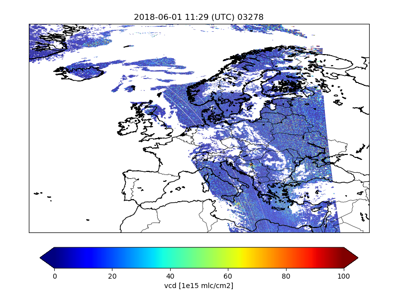
By default the catalogue creator simply creates a map with the value of the a variable on the track. Optionally settings could be used to specifiy a different unit, or the value range for the colorbar:
! convert units:
cso.tutorial.catalogue.var.vcd.units          :  1e15 mlc/cm2
! style:
cso.tutorial.catalogue.var.vcd.vmin           :   0.0
cso.tutorial.catalogue.var.vcd.vmax           :  10.0
Figures are saved to files with the basename of the original orbit file and the plotted variable:
/Scratch/CSO/catalogue/2018/06/01/S5p_RPRO_SO2_03278__vcd.png
                                  S5p_RPRO_SO2_03278__qa_value.png
                                  :
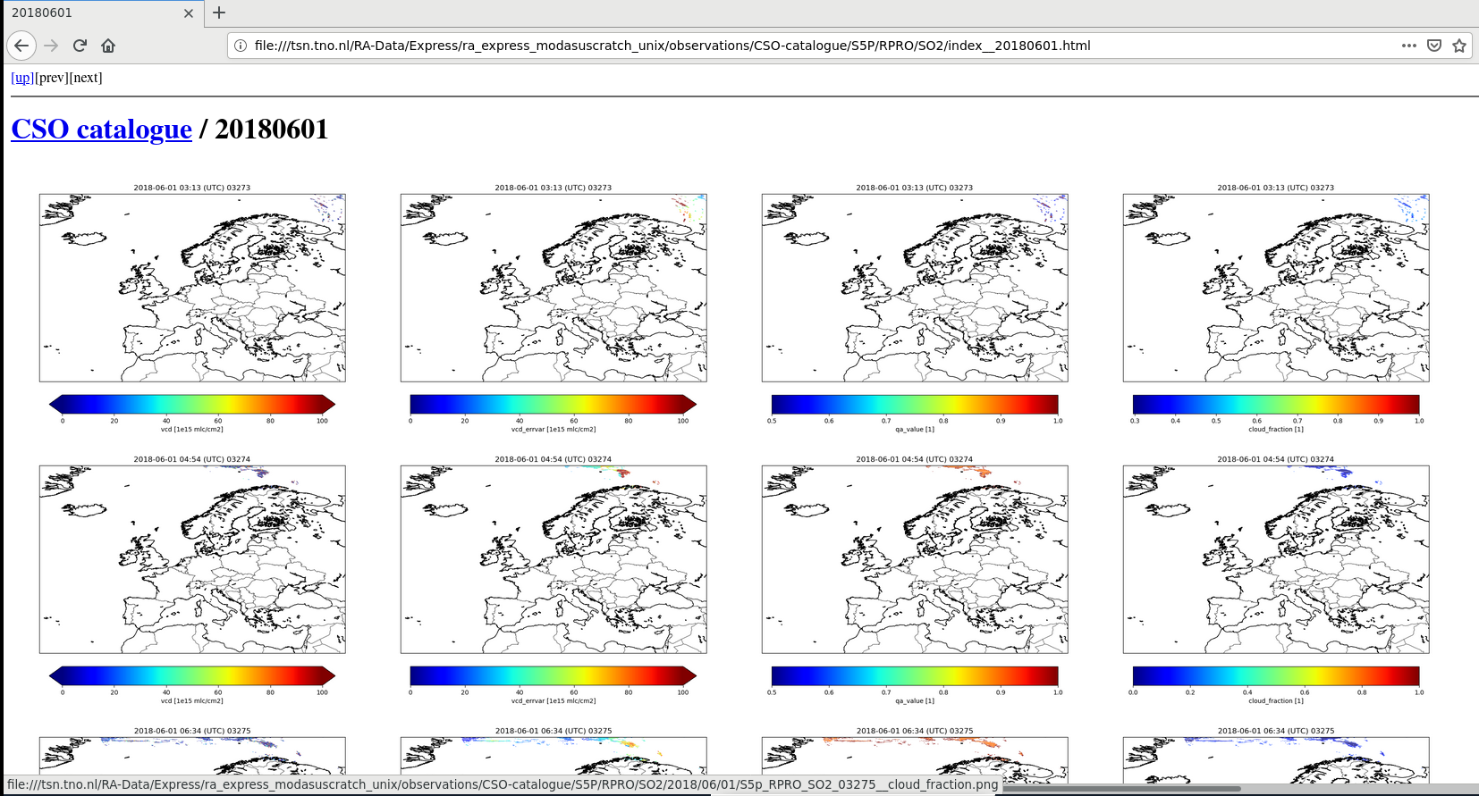
To search for interesting features in the data,
the Indexer class could be used to create index pages.
Configuration could look like:
! index creation task:
cso.s5p.so2.catalogue.task.index.class     :  utopya.Indexer
cso.s5p.so2.catalogue.task.index.args      :  '${PWD}/rc/cso-s5p-so2.rc', \
                                               rcbase='cso.s5p.so2.catalogue-index'
When succesful, the index creator displays an url that could be loaded in a browser:
Browse to:
  file:///Scratch/CSO/catalogue/index.html
Configuration of observation operator
The observation operator described in chapter ‘Observation operator’ requires settings from an rcfile.
First specify the (relative) location of the listing file with orbit file names and time ranges:
! template for listing with converted files:
<rcbase>.listing           : ../S5p/RPRO/SO2/CAMS/listing.csv
The operator should read variables from the data files that are needed to simulate a retrieval from the model arrays. This includes for example the pressures that define the a priori layers, the averaging kernel, and for this product, the airmass factor and tropopause level. Specify a list of names for these variables:
! data variables:
tutorial.S5p.hcho.dvars             :  hp yr vr A nla
Example settings:
! half-level pressures:
!~ dimensions, copied from data file:
tutorial.S5p.hcho.dvar.hp.dims      :  layeri
!~ source variable:
tutorial.S5p.hcho.dvar.hp.source    :  pressure

! retrieval:
!~ dimensions, copied from data file:
tutorial.S5p.hcho.dvar.yr.dims      :  retr
!~ source variable:
tutorial.S5p.hcho.dvar.yr.source    :  vcd

! retrieval error covariance:
!~ dimensions, copied from data file:
tutorial.S5p.hcho.dvar.vr.dims      :  retr retr
!~ source variable:
tutorial.S5p.hcho.dvar.vr.source    :  vcd_errvar

! kernel:
!~ dimensions, copied from data file:
tutorial.S5p.hcho.dvar.A.dims       :  retr layer
!~ source variable:
tutorial.S5p.hcho.dvar.A.source     :  kernel_trop

! number of apriori layers in retrieval layer:
!~ dimensions, copied from data file:
tutorial.S5p.hcho.dvar.nla.dims     :  retr
!~ source variable:
tutorial.S5p.hcho.dvar.nla.source   :  nla
For the simulated values, also define a list of variable names that should be created:
! state varaiables to be put out from model:
tutorial.S5p.hcho.vars                         :  mod_conc mod_hp mod_tcc mod_cc hx ys shx
Example settings:
! model concentration profile:
!~ model layer dimension:
tutorial.S5p.hcho.var.mod_conc.dims            :  model_layer
!~ standard attributes:
tutorial.S5p.hcho.var.mod_conc.attrs           :  long_name units
tutorial.S5p.hcho.var.mod_conc.attr.long_name  :  model HCHO concentrations
tutorial.S5p.hcho.var.mod_conc.attr.units      :  ppb

! model hpentration profile:
!~ model layer interfaces:
tutorial.S5p.hcho.var.mod_hp.dims              :  model_layeri
!~ standard attributes:
tutorial.S5p.hcho.var.mod_hp.attrs             :  long_name units
tutorial.S5p.hcho.var.mod_hp.attr.long_name    :  model pressure at layer interfaces
tutorial.S5p.hcho.var.mod_hp.attr.units        :  Pa

! total cloud cover:
!~ no extra dimensions:
tutorial.S5p.hcho.var.mod_tcc.dims             :
!~ standard attributes:
tutorial.S5p.hcho.var.mod_tcc.attrs            :  long_name units
tutorial.S5p.hcho.var.mod_tcc.attr.long_name   :  total cloud cover
tutorial.S5p.hcho.var.mod_tcc.attr.units       :  1

! cloud cover profiles:
!~ model layer dimension:
tutorial.S5p.hcho.var.mod_cc.dims              :  model_layer
!~ standard attributes:
tutorial.S5p.hcho.var.mod_cc.attrs             :  long_name units
tutorial.S5p.hcho.var.mod_cc.attr.long_name    :  cloud cover
tutorial.S5p.hcho.var.mod_cc.attr.units        :  1

! model concentrations at apriori layers:
!~ apriori layers:
tutorial.S5p.hcho.var.hx.dims                  :  layer
!~ how computed:
tutorial.S5p.hcho.var.hx.formula               :  LayerAverage( hp, mod_hp, mod_conc )
tutorial.S5p.hcho.var.hx.formula_terms         :  hp: hp mod_hp: mod_hp mod_conc: mod_conc
!~ standard attributes:
tutorial.S5p.hcho.var.hx.attrs                 :  long_name units
tutorial.S5p.hcho.var.hx.attr.long_name        :  model simulations at apriori layers
tutorial.S5p.hcho.var.hx.attr.units            :  mol m-2

! simulated retrievals
!~ retrieval layers:
tutorial.S5p.hcho.var.ys.dims                  :  retr
!~ how computed:
tutorial.S5p.hcho.var.ys.formula               :  A x
tutorial.S5p.hcho.var.ys.formula_terms         :  A: A x: hx
!~ standard attributes:
tutorial.S5p.hcho.var.ys.attrs                 :  long_name units multiplication_factor_to_convert_to_molecules_percm2
tutorial.S5p.hcho.var.ys.attr.long_name        :  simulated retrieval
tutorial.S5p.hcho.var.ys.attr.units            :  mol m-2
tutorial.S5p.hcho.var.ys.attr.multiplication_factor_to_convert_to_molecules_percm2 : float: 6.022141e+19

! partial columns as sum over apriori layers
!~ retrieval layers:
tutorial.S5p.hcho.var.shx.dims                 :  retr
!~ how computed:
tutorial.S5p.hcho.var.shx.formula              :  PartialColumns( nla, x )
tutorial.S5p.hcho.var.shx.formula_terms        :  nla: nla x: hx
!~ standard attributes:
tutorial.S5p.hcho.var.shx.attrs                :  long_name units multiplication_factor_to_convert_to_molecules_percm2
tutorial.S5p.hcho.var.shx.attr.long_name       :  tropospheric column in local model
tutorial.S5p.hcho.var.shx.attr.units           :  mol m-2
tutorial.S5p.hcho.var.shx.attr.multiplication_factor_to_convert_to_molecules_percm2 : float: 6.022141e+19
Sim-Catalogue
The CSO_Catalogue class could be used
to create a catalogue of images for the converted files.
Configuration could look like:
! catalogue creation task:
cso.s5p.TRACER.sim-catalogue.task.class          :  cso.CSO_SimCatalogue
cso.s5p.TRACER.sim-catalogue.task.args           :  '${PWD}/rc/cso-s5p-TRACER.rc', \
                                                  rcbase='cso.s5p.TRACER.sim-catalogue'
The configuration describes where to find a listing file with orbits,
which variables should be plot, the colorbar properties, etc.
See CSO_SimCatalogue class description for how
the settings in general look like.
The class creates figures for a list of variables:
! variables to be plotted:
cso.s5p.so2.catalogue.vars                    :  yr ys
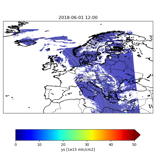
By default the catalogue creator simply creates a map with the value of the a variable on the track. Optionally settings could be used to specifiy a different unit, or the value range for the colorbar:
! variable:
cso.s5p.so2.sim-catalogue.var.yr.source          :  data:vcd
! convert units:
cso.s5p.so2.sim-catalogue.var.yr.units           :  1e15 mlc/cm2
! style:
cso.s5p.so2.sim-catalogue.var.yr.vmin            :   0.0
cso.s5p.so2.sim-catalogue.var.yr.vmax            :  50.0

! variable:
cso.s5p.so2.sim-catalogue.var.ys.source          :  state:y
! convert units:
cso.s5p.so2.sim-catalogue.var.ys.units           :  1e15 mlc/cm2
! style:
cso.s5p.so2.sim-catalogue.var.ys.vmin            :   0.0
cso.s5p.so2.sim-catalogue.var.ys.vmax            :  50.0
Figures are saved to files with the basename of the original orbit file and the plotted variable:
file://${my.run.base}/cso-catalogue/NO2//2018/06/01/S5p_RPRO_SO2_20180601_1200_yr.png
                                                    S5p_RPRO_SO2_20180601_1200_ys.png
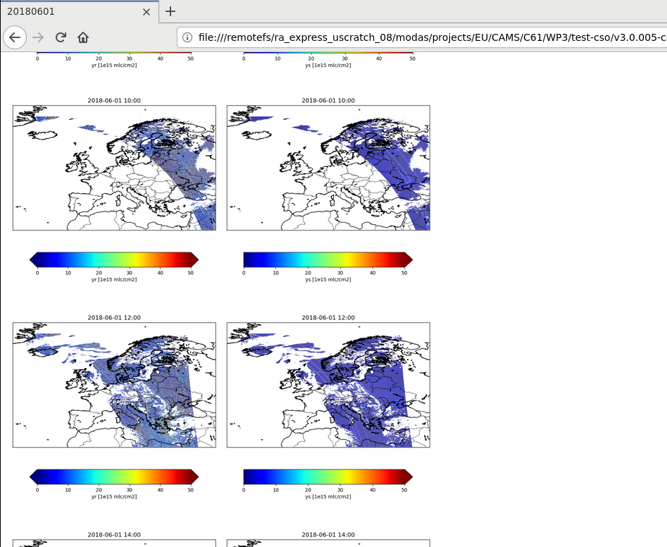
To search for interesting features in the data,
the Indexer class could be used to create index pages.
Configuration could look like:
! index creation task:
cso.s5p.so2.catalogue.task.index.class     :  utopya.Indexer
cso.s5p.so2.catalogue.task.index.args      :  '${PWD}/rc/cso-s5p-so2.rc', \
                                               rcbase='cso.s5p.so2.catalogue-index'
When succesful, the index creator displays an url that could be loaded in a browser:
Browse to:
  file://${my.run.base}/cso-catalogue/SO2/index__20180601.html
References
- Fioletov, V., McLinden, C. A., Griffin, D., Theys, N., Loyola, D. G., Hedelt, P., Krotkov, N. A., and Li, C.:Anthropogenic and volcanic point source SO2 emissions derived from TROPOMI on board Sentinel-5 Precursor: first results,Atmos. Chem. Phys., 20, 5591-5607, doi:10.5194/acp-20-5591-202, 2020.
- Theys, N., Hedelt, P., De Smedt, I. et al.Global monitoring of volcanic SO2 degassing with unprecedented resolution from TROPOMI onboard Sentinel-5 Precursor.Sci Rep 9, 2643 (2019). doi:10.1038/s41598-019-39279-y
Acknowledgements
We hereby thank D. Griffin and V. Fioletov for their valuable input.